Sergey Tomin (sergey.tomin@desy.de). January 2025.
An Introduction to Ocelot
Ocelot is a multiphysics simulation toolkit designed for studying Free Electron Lasers (FEL) and storage ring-based light sources. Implemented in Python, Ocelot caters to researchers seeking the flexibility provided by high-level languages like Matlab and Python. Its core principle revolves around scripting beam physics simulations in Python, utilizing Ocelot's modules and extensive collection of Python libraries.
Users developing high-level control applications can accelerate development by using physics models from Ocelot and Python graphics libraries such as PyQt and PyQtGraph to create a GUI.
Developing machine learning (ML) applications for accelerators can also benefit from using Ocelot, as many popular ML frameworks are written in Python. Ocelot provides a seamless connection between physics and ML methods, making it easier to integrate physical accelerator simulators with machine learning algorithms.
Documentation was generated automatically with the help of ChatGPT and has not yet been thoroughly reviewed or fully completed. The best and most reliable way to understand Ocelot remains reading the source code and docstrings for its functions and classes. Over time, we will continue to improve this documentation.
Requirements
- Python 3.9+
numpyversion 1.8 or higherscipyversion 0.15 or highermatplotlibversion 1.5 or higherh5pyversion 3.10 or higher
Orbit Correction module is required
Optional, but highly recommended for speeding up calculations
Installation
1. Install via Anaconda Cloud
To install OCELOT using Anaconda Cloud, run:
conda install -c ocelot-collab ocelot
This will install the latest stable version along with all required dependencies.
2. Install via PyPI
You can also install OCELOT from PyPI:
pip install ocelot-collab
ℹ️ The package name on PyPI is
ocelot-collab, but in Python you import it as:
>>> import ocelot
initializing ocelot...
>>> ocelot.__version__
'25.07.0'
3. Install from Source (Advanced)
To install OCELOT directly from GitHub:
 git clone https://github.com/ocelot-collab/ocelot.git
 cd ocelot
 python setup.py install
Alternatively, download the latest release as a ZIP file, unpack it, and install manually.
Getting Started: Simplest Accelerator Structure
Importing Ocelot Modules
The easiest way to import Ocelot is by using:
from ocelot import *
initializing ocelot...
Creating a Simple Lattice
Ocelot’s element syntax is similar to MAD8. Below, we create a simple lattice using quadrupoles, drift spaces, and a bending magnet (Bend). A beamline is simply a sequence of elements arranged in the correct order:
d = Drift(l=1)
qf = Quadrupole(l=0.3, k1=1)
qd = Quadrupole(l=0.3, k1=-1)
b = Bend(l=0.5, angle=0.1)
m1 = Marker(eid="start")
m2 = Marker(eid="stop")

cell = (m1, d, qf, d, qd, d, b,  d, qd, d, qf, d, m2)
The element sequence is then inserted into a MagneticLattice object, which acts as an abstraction layer between the sequence and other Ocelot functions, adding useful functionalities:
lat = MagneticLattice(cell)
print(f"total length {lat.totalLen}")
total length 7.699999999999999
Calculating Twiss Parameters
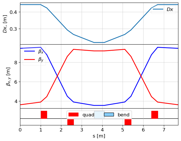
Twiss parameters can be calculated using the twiss() function. If initial Twiss parameters are not provided, the function will attempt to find a periodic solution:
tws = twiss(lat)
The twiss function returns a list of Twiss objects, each containing various beam parameters. To display key parameters of the first Twiss object:
print(tws[0])
    emit_x  = 0.0
    emit_y  = 0.0
    beta_x  = 9.449063560593697
    beta_y  = 3.6255987161054097
    alpha_x = -1.4029614496300944e-16
    alpha_y = -2.4207554851521635e-16
    gamma_x = 0.10583059300927898
    gamma_y = 0.27581651426504045
    Dx      = 0.4431890150023444
    Dy      = 0.0
    Dxp     = 4.152686605616285e-17
    Dyp     = 0.0
    mux     = 0.0
    muy     = 0.0
    nu_x    = 0.0
    nu_y    = 0.0
    E       = 0.0
    s        = 0.0
Plotting Twiss Parameters
Twiss parameters can be plotted using matplotlib or Ocelot a built-in function. It requires to import the graphical module separately.
This separation was implemented to decouple graphical libraries from calculations, which was necessary due to limitations in older computing clusters.
from ocelot.gui import *
plot_opt_func(lat, tws)
plt.show()

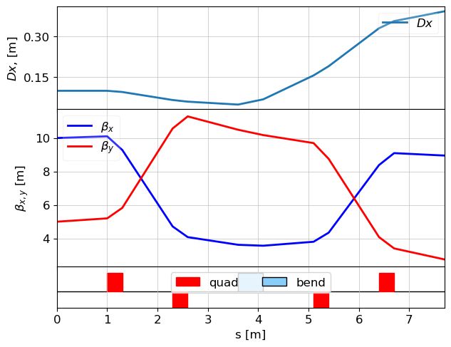
Specifying Initial Twiss Parameters
If known, initial Twiss parameters can be passed as an argument tws0:
tws0 = Twiss(beta_x = 10, beta_y=5, Dx=0.1)
tws = twiss(lat, tws0=tws0)

plot_opt_func(lat, tws)
plt.show()

More examples can be found in Tutorials
Disclaimer:
The OCELOT code comes with absolutely NO warranty. The authors of the OCELOT do not take any responsibility for any damage to equipments or personnel injury that may result from the use of the code.