Sergey Tomin (sergey.tomin@desy.de). June 2025.

TDCavity – Transverse Deflecting Cavity Element

The TDCavity class represents a Transverse Deflecting Structure (TDS) or cavity. It is primarily used to calculate the first-order transfer matrix for a beam passing through it. This matrix describes how the phase space coordinates of particles change as they traverse the cavity. By default, the cavity provides a horizontal kick, but this can be rotated using the tilt parameter.

Class Definition Snippet

from ocelot.cpbd.elements import TDCavity

# Example instantiation with default parameters (most are zero)
tds = TDCavity(l=0.1, freq=3e9, phi=0.0, v=0.01)  # 10 cm, S-band, 0 phase, 10 MV

# Full parameter list:
# tds = TDCavity(l=0., freq=0.0, phi=0.0, v=0., tilt=0.0, eid=None)

---

Parameters

• l (float): Nominal physical length of the cavity [m]. Used to scale the voltage if the actual segment length z differs from l.
• v (float): Total peak RF voltage across the nominal length l [GV]. Scaled for any segment as: $$V_{\text{segment}} = v \cdot \frac{z}{l}$$
• freq (float): Operating RF frequency [Hz].
• phi (float): RF phase [degrees]. Conventionally:
  • $\phi = 0^\circ$: zero-crossing (maximum transverse kick)
  • $\phi = 90^\circ$: on-crest (maximum energy gain for accelerating cavities)
• tilt (float, optional): Rotation angle in the transverse plane around the beam axis [rad]. A value of 0 implies horizontal kick; $\pi/2$ gives vertical.
• eid (str, optional): Element identifier.

---

Transfer Matrix Formulation

The TDCavity element generates a $6 \times 6$ transfer matrix $R$ that describes the linear transformation of a particle’s 6D phase space vector through the cavity.

Ocelot Coordinate System

Ocelot uses the following 6D phase space convention:

$$(x, \quad x' = \frac{p_x}{p_0}), \quad (y, \quad y' = \frac{p_y}{p_0}), \quad (\tau = c\Delta t, \quad \delta = \frac{\Delta E}{p_0 c})$$

In code, the 6th coordinate is often labeled p, but here we use $\delta$ to clearly denote the relative energy deviation.

The matrix is computed by:

tds_R_z(z, energy, freq, v, phi)

• segment length z [m]
• total reference energy [GeV]
• RF frequency [Hz]
• scaled voltage [GV]
• phase [deg]

---

R-Matrix for Horizontal Deflection

The resulting matrix for a horizontally deflecting cavity segment of length $z$ is:

$$R_{\text{code}}(z) = \begin{bmatrix} 1 & z & 0 & 0 & -\frac{z}{2} K \cos(\phi) & 0 \\ 0 & 1 & 0 & 0 & -K \cos(\phi) & 0 \\ 0 & 0 & 1 & z & 0 & 0 \\ 0 & 0 & 0 & 1 & 0 & 0 \\ 0 & 0 & 0 & 0 & 1 & -\frac{z}{\gamma^2 -1 } \\ K \cos(\phi) & \frac{z}{2} K \cos(\phi) & 0 & 0 & -\frac{z}{6} K^2 \cos(2\phi) & 1 \end{bmatrix}$$

Where:

• $K = \dfrac{V_{\text{seg}} \cdot k_0}{p_0 c}$ — normalized TDS strength (dimensionless)
• $k_0 = \dfrac{2\pi f}{c}$ — RF wavenumber [1/m]
• $p_0 c = m_e c^2 \sqrt{\gamma^2 - 1}$ — reference momentum-energy [GeV]
• $\gamma = \dfrac{E_{\text{ref}}}{m_e c^2}$ — Lorentz factor

The matrix is later rotated if a tilt is applied.

---

Application: Induced Slice Energy Spread

Due to the Panofsky–Wenzel theorem, a transverse deflecting field with time (or longitudinal position) dependence must be accompanied by a longitudinal field component depending on transverse coordinates. This results in an induced energy deviation across the bunch [1, 2].

The relative energy deviation of the central slice ($\tau = 0$) at the cavity exit is:

$$\delta_f = \delta_0 + R_{61} x_0 + R_{62} x_0' + R_{66} \delta_0$$

With $R_{66} = 1$ and defining $a = K \cos\phi$, we get:

$$\Delta \delta = \delta_f - \delta_0 = a x_0 + \frac{z}{2} a x_0'$$

So the new energy deviation becomes:

$$\delta_1 = \delta_0 + \Delta \delta$$

RMS Energy Spread

We compute the final slice energy spread:

$$\sigma_\delta^2 = \langle \delta_1^2 \rangle - \langle \delta_1 \rangle^2$$

Assuming:

• $\langle x_0 \rangle = \langle x_0' \rangle = \langle \delta_0 \rangle = 0$ - the beam does not have any offsets.
• $\langle \delta_0 x_0 \rangle = \langle \delta_0 x_0' \rangle = 0$ - there are no correlations in the beam between energy and transverse coordinates.

We obtain:

$$\sigma_\delta^2(z) = \langle \delta_0^2 \rangle + a^2 \langle x_0^2 \rangle + z a^2 \langle x_0 x_0' \rangle + \frac{z^2 a^2}{4} \langle (x_0')^2 \rangle$$

Using Twiss Parameters:

• $\langle x_0^2 \rangle = \varepsilon_x \beta_x$
• $\langle x_0 x_0' \rangle = -\varepsilon_x \alpha_x$
• $\langle (x_0')^2 \rangle = \varepsilon_x \gamma_x^{\text{Twiss}}$

Then the induced energy spread from the TDS becomes:

$$(\sigma_\delta^2)_{\text{TDS}} = a^2 \varepsilon_x \left( \beta_x - z \alpha_x + \frac{z^2}{4} \gamma_x^{\text{Twiss}} \right)$$

Or:

$$(\sigma_\delta)_{\text{TDS}} = |K \cos\phi| \cdot \sqrt{ \varepsilon_x \left( \beta_x(0) - z \alpha_x(0) + \frac{z^2}{4} \gamma_x^{\text{Twiss}}(0) \right) }$$

Note: Here, $\gamma$ (no subscript) is the relativistic Lorentz factor, while $\gamma_x^{\text{Twiss}}$ is the Twiss parameter.

This expression was used in [3].

---

References

1. S.Korepanov et al, AN RF DEFLECTOR FOR THE LONGITUDINAL AND TRANSVERSE BEAM PHASE SPACE ANALYSIS AT PITZ
2. C. Behrens and C. Gerth, ON THE LIMITATIONS OF LONGITUDINAL PHASE SPACE MEASUREMENTS USING A TRANSVERSE DEFLECTING STRUCTURE
3. S.Tomin et al, Accurate measurement of uncorrelated energy spread in electron beam, Phys. Rev. Accel. Beams 24, 064201

Summary

The TDCavity provides a time-dependent transverse kick to the beam. According to the Panofsky–Wenzel theorem, this results in a correlated longitudinal effect, increasing the slice energy spread.

Examples of Use

1. Basic Instantiation and Transfer Matrix Calculation

import numpy as np
from ocelot.cpbd.elements import TDCavity

import numpy as np
from ocelot.cpbd.elements import TDCavity

# Create a TDCavity element: 1 meter long, S-band frequency, 0° phase, 30 MV voltage
tds = TDCavity(l=1.0, freq=3e9, phi=0.0, v=0.03)

# Print the first-order transfer matrix at 1 GeV
np.set_printoptions(precision=3, suppress=True)
print(tds.R(energy=1.0))  # [GeV]

    [array([[ 1.   ,  1.   ,  0.   ,  0.   , -0.943,  0.   ],
           [ 0.   ,  1.   ,  0.   ,  0.   , -1.886,  0.   ],
           [ 0.   ,  0.   ,  1.   ,  1.   ,  0.   ,  0.   ],
           [ 0.   ,  0.   ,  0.   ,  1.   ,  0.   ,  0.   ],
           [ 0.   ,  0.   ,  0.   ,  0.   ,  1.   , -0.   ],
           [ 1.886,  0.943,  0.   ,  0.   , -0.593,  1.   ]])]

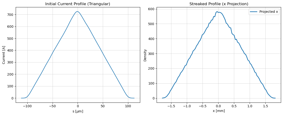
Tracking with TDS: Visualizing the Current Profile

In this example, we demonstrate how a Transverse Deflecting Cavity (TDS) can be used to convert the longitudinal structure of a bunch into a transverse streak, making it observable on a screen.

We generate a particle distribution with a triangular current profile and propagate it through a simple beamline that includes a TDS. The final transverse (x) distribution at the exit should mirror the original current shape, allowing us to confirm the streaking effect.

⚠️ In this example, we are only interested in the shape of the profile, not its absolute amplitude.

We use:

• MagneticLattice to define the beamline,
• ParticleArray class,
• Twiss class,
• generate_parray() to generate the particle distribution,
• and track() function for ParticleArray tracking.

If you're interested in more details about how the TDS works and its impact on beam diagnostics, see this Optics for High Time Resolution Measurements with TDS.

from ocelot import *
from ocelot.gui import *
# Define TDS and lattice
tds = TDCavity(l=1.0, freq=3e9, phi=0.0, v=0.03)
d = Drift(l=1.0)
qf = Quadrupole(l=0.2, k1=1.0)
qd = Quadrupole(l=0.2, k1=-1.0)
lat = MagneticLattice([tds, d] + list((qf, d, qd, d) * 4))

# Define initial Twiss parameters
tws0 = Twiss(beta_x=10, beta_y=10, alpha_x=-1, alpha_y=0.8, emit_xn=1e-6, emit_yn=1e-6, E=1.0)

# Generate triangular-shaped longitudinal distribution
parray = generate_parray(tws=tws0, charge=250e-12, sigma_p=1e-4,
                         chirp=0, sigma_tau=1e-4, nparticles=500_000, shape="tri")

# Initial current profile
plt.figure(figsize=(12, 5))
plt.subplot(1, 2, 1)
current_profile = parray.I()
plt.plot(current_profile[:, 0]*1e6, current_profile[:, 1])
plt.title("Initial Current Profile (Triangular)")
plt.xlabel(r"s [$\mu$m]")
plt.ylabel("Current [A]")

# Track particles through the lattice (TDS will convert τ → x)
track(lat, parray)

# Plot streaked distribution (projected on x)
plt.subplot(1, 2, 2)
counts, bin_edges = np.histogram(parray.x(), bins=100, density=True)
bin_centers = 0.5 * (bin_edges[:-1] + bin_edges[1:])
plt.plot(bin_centers*1e3, counts, label="Projected x", linewidth=2)
plt.title("Streaked Profile (x Projection)")
plt.xlabel("x [mm]")
plt.ylabel("Density")
plt.grid(True)
plt.legend()
plt.tight_layout()
plt.show()

    [INFO    ] Twiss parameters have priority. sigma_{x, px, y, py} will be redefined


    z = 11.599999999999998 / 11.599999999999998. Applied: 

3. Slice Energy Spread Growth Due to TDS

In this example, we illustrate how the Transverse Deflecting Structure (TDS) increases the slice energy spread due to the Panofsky–Wenzel effect, and compare the result with the analytical prediction derived earlier.

📌 Note: The slice energy spread should be evaluated in a narrow time window around $\tau = 0$, as assumed in the derivation above. This ensures the comparison with theory is valid.

SIGMA_P = 1e-4
# Generate fresh distribution without triangular shape
parray = generate_parray(tws=tws0, charge=250e-12, sigma_p=1e-4,
                         chirp=0, sigma_tau=SIGMA_P, nparticles=500_000)

# Track through lattice
track(lat, parray)

# Compute energy spread from particle distribution in a small slice
sigma_p_measured = np.sqrt(parray.get_twiss(bounds=[-0.1, 0.1]).pp)
print(f"Measured σ_p from slice: {sigma_p_measured:.3e}")

# Analytical estimate using Panofsky-Wenzel formulation
Ktds = tds.v * 2 * np.pi * tds.freq / (parray.E * speed_of_light)
sigma_E_tds = Ktds * np.cos(tds.phi) * np.sqrt(
    tws0.emit_x * (tws0.beta_x - tds.l * tws0.alpha_x + (tds.l**2 / 4) * tws0.gamma_x)
)
sigma_total = np.sqrt((SIGMA_P)**2 + sigma_E_tds**2)

print(f"Analytical σ_p after TDS: {sigma_total:.3e}")

    [INFO    ] Twiss parameters have priority. sigma_{x, px, y, py} will be redefined


    z = 11.599999999999998 / 11.599999999999998. Applied: 
    Measured σ_p from slice: 1.734e-04
    Analytical σ_p after TDS: 1.735e-04