This notebook was created by Sergey Tomin (sergey.tomin@desy.de). June 2019.

1. Synchrotron Radiation Module

OCELOT includes a native Python synchrotron-radiation (SR) module. It combines Runge-Kutta particle tracking with a frequency-domain radiation solver.

This tutorial introduces spontaneous-radiation spectra and spatial distributions for a single electron. Magnetic fields can be supplied through an ideal Undulator, an on-axis or three-dimensional field map, or a Python magnetic-field function. The beam current is used to normalize the result as photon flux.

The numerical method and applications are described in S. Tomin and G. Geloni, Synchrotron Radiation Module in OCELOT Toolkit, IPAC 2019, WEPTS017.

Contents

1. Ideal magnetic field
   • Spatial distribution
     • Phase
   • Spectrum
   • 3D spatial distribution
2. Magnetic field map on the undulator axis
3. Radiation from a bending magnet

Ideal magnetic field

For an ideal planar undulator, use a sinusoidal vertical magnetic field

$$B_y(x, y, z) = B_0 \sin\left(\frac{2\pi z}{\lambda_u}\right)$$

with $B_x(x, y, z) = B_z(x, y, z) = 0$. This field is represented by an Undulator element configured with $K$, the period length, and the number of periods.

# To activate interactive Matplotlib in the notebook
#%matplotlib notebook

# Import the main functions from the synchrotron-radiation (SR) module
from ocelot.rad import *
# import OCELOT main functions 
from ocelot import *
# import OCELOT plotting functions 
from ocelot.gui import *
import time

We begin by creating an element and a magnetic lattice.

The radiation module treats Undulator as the radiating element. Other lattice elements can be included for particle tracking, but they do not automatically provide a magnetic field to the radiation integrator. An arbitrary field, including a dipole-like field, can be supplied through Undulator.mag_field, as shown later in this tutorial.

und = Undulator(Kx=0.43, nperiods=500, lperiod=0.007, eid="und")

lat = MagneticLattice((und))

The radiation calculation uses two additional objects:

• Beam() provides the electron energy, initial coordinates, and beam current. The trajectory and field are calculated for one electron; the current normalizes the result to photons per second.

warning

calculate_radiation calculates the field from one electron trajectory. Beam emittance and energy-spread averaging are not performed by this function.

• Screen() defines the observation geometry and photon-energy grid and stores the calculated fields and photon distributions.

Spatial distribution

To calculate a spatial distribution, define the screen size and the number of points in each transverse plane. We start with the simplest one-dimensional case.

beam = Beam()
beam.E = 2.5            # beam energy in [GeV]
beam.I = 0.1            # beam current in [A]


screen = Screen()
screen.z = 100.0      # distance from the beginning of lattice to the screen
screen.size_x = 0.002 # half of screen size in [m] in horizontal plane
screen.size_y = 0.    # half of screen size in [m] in vertical plane
screen.nx = 101       # number of points in horizontal plane 
screen.ny = 1         # number of points in vertical plane 


screen.start_energy = 7761.2 # [eV], starting photon energy
screen.end_energy = 7900     # [eV], ending photon energy
screen.num_energy = 1        # number of energy points[eV]

Calculate SR

Use the following function to calculate spontaneous radiation from one electron:

screen = calculate_radiation(lat, screen, beam)

• lat: MagneticLattice containing at least one nonzero-length radiating element
• screen: observation Screen
• beam: Beam supplying the electron coordinates, energy, and current

Optional parameters:

• energy_loss=False: apply one aggregate classical energy correction per undulator
• quantum_diff=False: apply a stochastic energy correction per undulator
• accuracy=1: scale the automatically estimated trajectory-point count

For exact trajectory sampling, specify npoints on the Undulator or its Runge-Kutta transformation. An explicit npoints value overrides accuracy. End-pole behavior is configured on the Undulator element rather than passed to calculate_radiation.

start = time.time()
screen = calculate_radiation(lat, screen, beam)
print("time exec: ", time.time() - start, " sec")

The electric-field components are stored in one-dimensional arrays with logical order (energy, y, x):

• screen.arReEx: real part of the horizontal field
• screen.arImEx: imaginary part of the horizontal field
• screen.arReEy: real part of the vertical field
• screen.arImEy: imaginary part of the vertical field
• screen.arPhase: accumulated phase

The Screen also stores the coordinates at which the radiation was calculated:

• screen.Xph: horizontal coordinates
• screen.Yph: vertical coordinates
• screen.Eph: photon energies

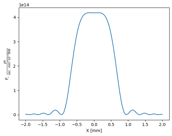
Photon flux is calculated from the electric field and stored in 1D arrays:

• screen.Sigma: horizontal polarization component in $\left[\frac{ph}{sec \cdot mm^2 \cdot 10^{-3}BW}\right]$
• screen.Pi: vertical polarization component in $\left[\frac{ph}{sec \cdot mm^2 \cdot 10^{-3}BW}\right]$
• screen.Total = screen.Sigma + screen.Pi: total flux density in $\left[\frac{ph}{sec \cdot mm^2 \cdot 10^{-3}BW}\right]$

Here 10^-3 BW denotes a relative photon-energy bandwidth $\Delta E/E = 10^{-3}$, not the spacing between adjacent samples in screen.Eph.

plt.figure(10)
plt.plot(screen.Xph, screen.Total)
plt.ylabel(r"F, $\frac{ph}{sec \cdot mm^2 10^{-3}BW}$")
plt.xlabel(r"X [mm]")
plt.show()

Plotting utilities

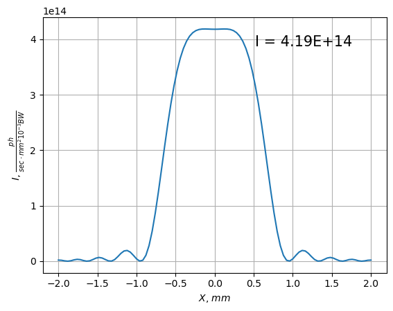
Use the standard plotting function:

show_flux(screen, unit="mm")

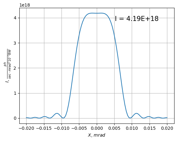
Angular coordinates in [mrad]

show_flux(screen, unit="mrad",  nfig=2)

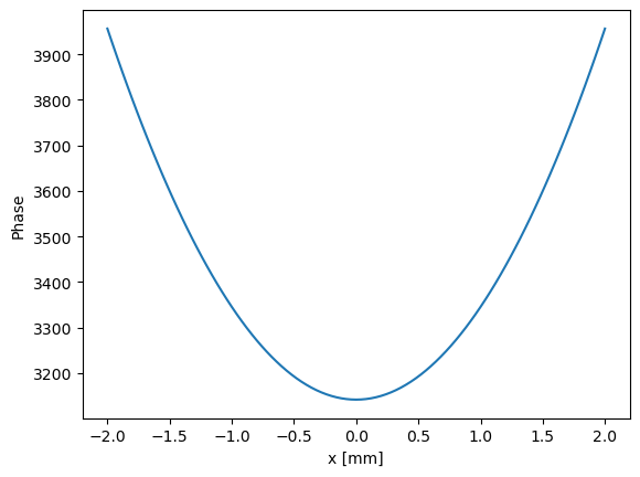
Phase

Relation between the time $\tau$ at the observer and the time $t$ of emission

$$\tau(t) = t + \frac{1}{c}\big|\vec{x_{scr}} - \vec{r(t)}\big| = \tau_0 + \int_0^t{\left[1 - \vec{n(t')} \vec{\beta(t')} \right]dt'}$$

where $\vec{x_{scr}} = [x_{scr}, y_{scr}, z_{scr}]$

$$\phi(z, \vec{x_{scr}}) = \frac{2\pi c}{\lambda}\tau(t(z)) = \frac{2\pi }{\lambda}\left(c t(z) + \big|\vec{x_{scr}} - \vec{r(z)}\big|\right)$$ $$\phi(z, \vec{x_{scr}}) = \phi(z_0, \vec{x_{scr}}) + \frac{2\pi }{\lambda}\int_{z_0}^z{\frac{dz'}{\sqrt{\beta^2 - \beta^2_x(z') - \beta_y^2(z')}}} + \frac{2\pi }{\lambda}\big|\vec{x_{scr}} - \vec{r(z)}\big| - \frac{2\pi }{\lambda}\big|\vec{x_{scr}} - \vec{r(z_0)}\big|$$

where

$$\phi(z_0, \vec{x_{scr}}) = \frac{2\pi c }{\lambda} t(z_0)+ \frac{2\pi }{\lambda}\big|\vec{x_{scr}} - \vec{r(z_0)}\big|$$

$\vec{r(z)}= [x(z), y(z), z]$ is the electron trajectory,

Using assumptions:

$$\begin{aligned} &\gamma >> 1, \qquad |\beta_x|<< 1, \qquad |\beta_y|<<1 \\ (z_{scr} - z_0) >> (z - z_0), &\qquad (z_{scr} - z_0) >> (x_{scr} - x(z)), \qquad (z_{scr} - z_0) >> (y_{scr} - y(z)) \end{aligned}$$

we finally get

$$\begin{aligned} \phi(z, \vec{x_{scr}}) = \phi(z_0, \vec{x_{scr}}) + \frac{\pi}{\lambda \gamma^2}\left[(z - z_0) + \gamma^2 \int_{z_0}^z\left\{\beta_x^2(z') + \beta_y^2(z')\right\}dz' + \gamma^2 \left[\frac{(x_{scr} - x(z))^2}{z_{scr} - z} - \frac{(x_{scr} - x(z_0))^2}{z_{scr} - z_0}\right] + \gamma^2 \left[\frac{(y_{scr} - y(z))^2}{z_{scr} - z} - \frac{(y_{scr} - y(z_0))^2}{z_{scr} - z_0}\right]\right] \end{aligned}$$

During the trajectory integration, the reference phase is taken as $\phi(z_0, \vec{x_{scr}}) = 0$.

At the end of calculate_radiation, screen.rebuild_efields(x0, y0, z0) restores the initial geometric phase term using the starting point of the electron trajectory.

plt.figure(1000)
plt.plot(screen.Xph, screen.arPhase)
plt.xlabel("x [mm]")
plt.ylabel("Phase")
plt.show()

Spectrum

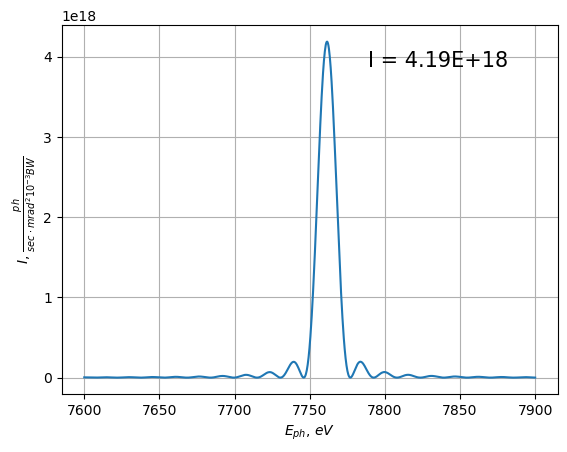
The on-axis spectrum is calculated in the same way, using one transverse screen point and a photon-energy grid.

beam = Beam()
beam.E = 2.5            # beam energy in [GeV]
beam.I = 0.1            # beam current in [A]


screen = Screen()
screen.z = 100.0      # distance from the beginning of lattice to the screen


screen.start_energy = 7600     # [eV], starting photon energy
screen.end_energy = 7900       # [eV], ending photon energy
screen.num_energy = 1000       # number of energy points[eV]

# Calculate radiation 
start = time.time()
screen = calculate_radiation(lat, screen, beam)
print("time exec: ", time.time() - start, " sec")

# show result
show_flux(screen, unit="mrad",  nfig=12)

2D spatial distribution

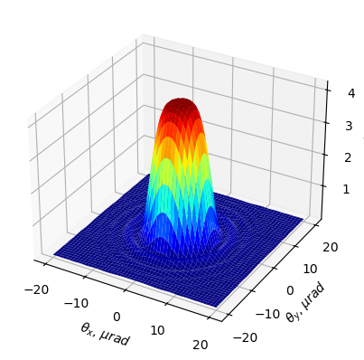
beam = Beam()
beam.E = 2.5            # beam energy in [GeV]
beam.I = 0.1            # beam current in [A]


screen = Screen()
screen.z = 100.0        # distance from the beginning of lattice to the screen
screen.size_x = 0.002   # half of screen size in [m] in horizontal plane
screen.size_y = 0.002   # half of screen size in [m] in vertical plane
screen.nx = 51          # number of points in horizontal plane 
screen.ny = 51          # number of points in vertical plane 


screen.start_energy = 7761.2 # [eV], starting photon energy
screen.end_energy = 7900     # [eV], ending photon energy
screen.num_energy = 1        # number of energy points[eV]

start = time.time()

# Calculate radiation 
screen = calculate_radiation(lat, screen, beam)
print("time exec: ", time.time() - start, " sec")

# show result
show_flux(screen, unit="mrad",  nfig=13)

3D distribution in arbitrary domains

See PFS tutorial N4: Converting synchrotron-radiation results from a Screen object to RadiationField.

Magnetic-field map on the undulator axis

Spatial coordinates in field-map files are expressed in millimetres. Three formats are supported:

1. Planar undulator: two columns, [z, By], with $z$ in mm and $B_y$ in T.
2. Helical undulator: three columns, [z, Bx, By], with $z$ in mm and field components in T.
3. Three-dimensional map: [x, y, z, Bx, By, Bz].

Planar undulator

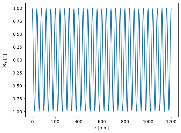
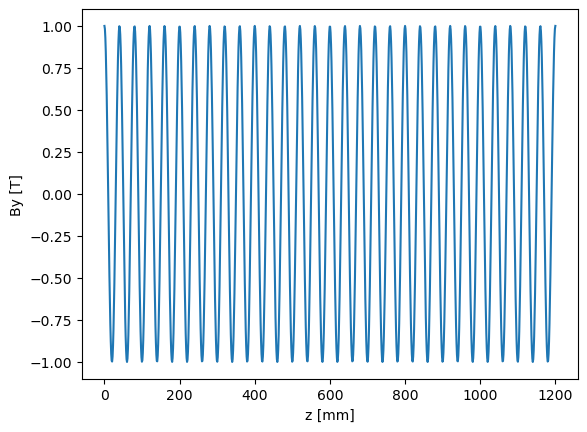
First, generate an on-axis magnetic field.

lperiod = 0.04 # [m] undulator period 
nperiods = 30  # number of periods
B0 = 1         # [T] amplitude of the magnetic field

# longitudinal coordinates from 0 to lperiod*nperiods in [mm] 
z = np.linspace(0, lperiod*nperiods, num=500)*1000 # [mm] 
lperiod_mm = lperiod * 1000 # in [mm]
By = B0*np.cos(2*np.pi/lperiod_mm*z)

plt.figure(100)
plt.plot(z, By)
plt.xlabel("z [mm]")
plt.ylabel("By [T]")
plt.show()

Save the map into a file

filed_map = np.vstack((z, By)).T

np.savetxt("filed_map.txt", filed_map)

Create undulator element with field map and initialize MagneticLattice

und_m = Undulator(field_file="filed_map.txt", eid="und")

lat_m = MagneticLattice((und_m))

beam = Beam()
beam.E = 17.5            # beam energy in [GeV]
beam.I = 0.1            # beam current in [A]


screen = Screen()
screen.z = 1000.0      # distance from the beginning of lattice to the screen


screen.start_energy = 7000      # [eV], starting photon energy
screen.end_energy = 12000       # [eV], ending photon energy
screen.num_energy = 1000        # number of energy points[eV]

# Calculate radiation 
screen = calculate_radiation(lat_m, screen, beam)

# show result
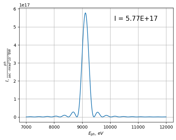
show_flux(screen, unit="mrad",  nfig=103)

Estimate radiation properties

Estimate basic radiation properties with:

print_rad_props(beam, K, lu, L, distance)

• beam is Beam class
• K is undulator parameter
• lu is undulator period in [m]
• L is undulator length in [m]
• distance is distance to the screen in [m]

Helper functions also convert between undulator parameters, for example:

field2K(field, lu=0.04)

K = field2K(field=B0, lu=lperiod)
print_rad_props(beam, K, lu=lperiod, L=lperiod*nperiods, distance=screen.z)

********* ph beam ***********
Ebeam        :  17.5  GeV
K            :  3.7349164279988596
B            :  1.0  T
lambda       :  1.35992E-10  m
Eph          :  9.11702E+03  eV
1/gamma      :  29.1999  um
sigma_r      :  1.4376  um
sigma_r'     :  7.5275  urad
Sigma_x      :  1.4376  um
Sigma_y      :  1.4376  um
Sigma_x'     :  7.5275 urad
Sigma_y'     :  7.5275 urad
H. spot size :  7.5275 / 0.0075  mm/mrad
V. spot size :  7.5275 / 0.0075  mm/mrad
I            :  0.1  A
Nperiods     :  30.0
distance     :  1000.0  m
flux tot     :  2.05E+14  ph/sec/0.1%BW
flux density :  5.76E+17  ph/sec/mrad^2/0.1%BW;    5.76E+11  ph/sec/mm^2/0.1%BW
brilliance   :  4.44E+22  ph/sec/mrad^2/mm^2/0.1%BW

K = field2K(field=B0, lu=lperiod)
beam = Beam()
beam.E = 0.13
beam.I = 0.1

print_rad_props(beam, K=20, lu=0.2, L=lperiod*20, distance=100)

********* ph beam ***********
Ebeam        :  0.13  GeV
K            :  20
B            :  1.071  T
lambda       :  3.10563E-04  m
Eph          :  3.99224E-03  eV
1/gamma      :  3930.7605  um
sigma_r      :  1773.8821  um
sigma_r'     :  13932.0371  urad
Sigma_x      :  1773.8821  um
Sigma_y      :  1773.8821  um
Sigma_x'     :  13932.0371 urad
Sigma_y'     :  13932.0371 urad
H. spot size :  1393.2048 / 13.932  mm/mrad
V. spot size :  1393.2048 / 13.932  mm/mrad
I            :  0.1  A
Nperiods     :  4.0
distance     :  100  m
flux tot     :  2.77E+13  ph/sec/0.1%BW
flux density :  2.27E+10  ph/sec/mrad^2/0.1%BW;    2.27E+06  ph/sec/mm^2/0.1%BW
brilliance   :  1.15E+09  ph/sec/mrad^2/mm^2/0.1%BW

Arbitrary magnetic field: Python function

OCELOT can define a three-dimensional magnetic field as a Python function.

We repeat the preceding field-map example using this approach.

lperiod = 0.04 # [m] undulator period 
nperiods = 30  # number of periods
B0 = 1         # [T] amplitude of the magnetic field

# longitudinal coordinates from 0 to lperiod*nperiods in [mm] 
z = np.linspace(0, lperiod*nperiods, num=1000)*1000 # [mm] 
By = B0*np.cos(2*np.pi/lperiod*z)


def py_mag_field(x, y, z, lperiod, B0):
    """
    x, y, z = coordinates
    """
    Bx = 0
    By = B0*np.cos(2*np.pi/lperiod*z)
    Bz = 0
    return (Bx, By, Bz)


plt.figure(110)
plt.plot(z, py_mag_field(x=0, y=0, z=z, lperiod=lperiod, B0=B0)[1])
plt.xlabel("z [mm]")
plt.ylabel("By [T]")
plt.show()

Attribute mag_field

An Undulator element can define an arbitrary magnetic field through the mag_field callable: (Bx, By, Bz) = f(x, y, z).

For example, define a vertical field while setting the other components to zero:

field = lambda x, y, z: (0, cos(kz * z), 0)

When mag_field is a function, lperiod and nperiods are still required because they define the element length.

und_m = Undulator(lperiod=lperiod, nperiods=nperiods, Kx=0.0,eid="und")
und_m.mag_field = lambda x, y, z: py_mag_field(x, y, z, lperiod=lperiod, B0=B0)

# next, all the same.

lat_m = MagneticLattice((und_m))


beam = Beam()
beam.E = 17.5            # beam energy in [GeV]
beam.I = 0.1            # beam current in [A]


screen = Screen()
screen.z = 1000.0      # distance from the beginning of lattice to the screen


screen.start_energy = 7000      # [eV], starting photon energy
screen.end_energy = 12000       # [eV], ending photon energy
screen.num_energy = 1000        # number of energy points[eV]

# Calculate radiation 
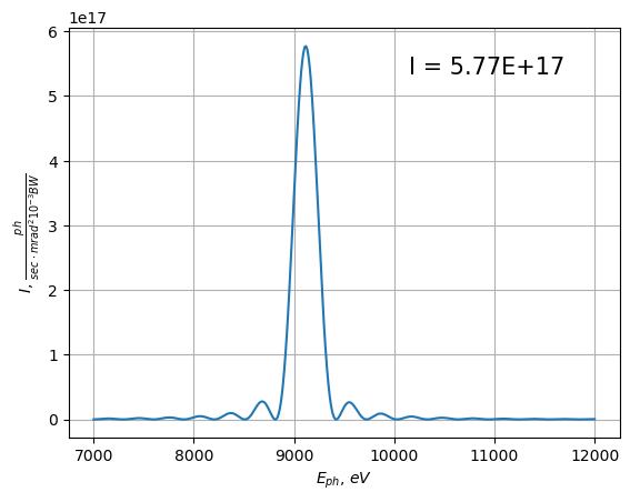
screen = calculate_radiation(lat_m, screen, beam, accuracy=2)

# show result
show_flux(screen, unit="mrad",  nfig=104)

Accuracy and number of trajectory points

If no explicit point count is supplied, calculate_radiation(..., accuracy=1) scales the automatically estimated number of trajectory points. For an undulator of length $L_u$ in metres, the current estimate is

n = int((L_u * 1500 + 100) * accuracy)

Set Undulator(..., npoints=N) or configure npoints on its Runge-Kutta transformation to request exactly $N$ points. Explicit npoints overrides accuracy and must be an integer of at least four.

Trajectory

After the radiation calculation, the Screen contains the trajectories used by the solver in a BeamTraject object:

screen.beam_traj = BeamTraject()

Specify the particle index to retrieve a trajectory, for example:

x = screen.beam_traj.x(n=0)

See Tutorial N9, Simple accelerator-based THz source, for a multi-particle example.

For calculate_radiation, BeamTraject contains one electron trajectory, so the valid particle index is n = 0.

n = 0
x = screen.beam_traj.x(n)
y = screen.beam_traj.y(n)
z = screen.beam_traj.z(n)
plt.title("trajectory of " + str(n)+"th particle")
plt.plot(z, x, label="X")
plt.plot(z, y, label="Y")
plt.xlabel("Z [m]")
plt.ylabel("X/Y [m]")
plt.legend()
plt.show()

print(f"Number of trajectory points n={len(z)}")

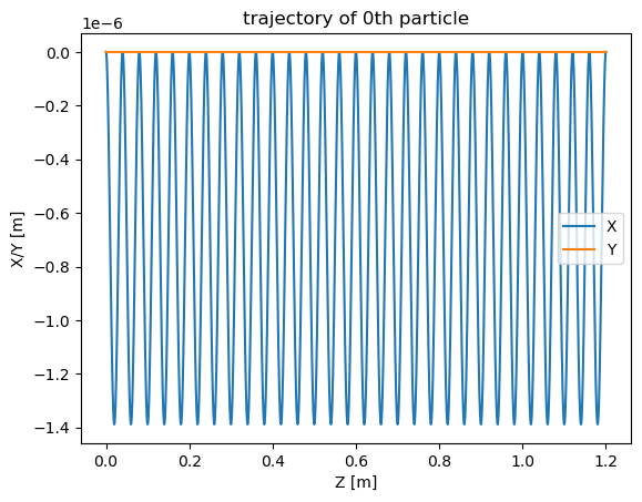
Number of trajectory points n=3800

Radiation from a bending magnet

The SR module does not directly use a Bend element as a radiating element. The same magnetic field can instead be represented by an Undulator with a custom field function, as demonstrated below.

We use the Undulator.mag_field callable to represent a uniform bending-magnet field.

Assume a vertical bending field with amplitude $B_y = 1\,\mathrm{T}$.

By = 1. # T - amplitude of vertical magnetic field. 

b = Undulator(lperiod=0.10, nperiods=10, eid="und")
b.mag_field = lambda x, y, z: (0, By, 0)

# in the Undulator element parameters lperiod and nperiods are needed 
# just for definition of the length of the element
d = Drift(l=1)
lat_b = MagneticLattice((b,))


beam = Beam()
beam.E = 2            # beam energy in [GeV]
beam.I = 0.1            # beam current in [A]


screen = Screen()
screen.z = 1000.0      # distance from the beginning of lattice to the screen


screen.start_energy = 100      # [eV], starting photon energy
screen.end_energy = 20000       # [eV], ending photon energy
screen.num_energy = 1000        # number of energy points[eV]

# Calculate radiation 
start = time.time()
screen = calculate_radiation(lat_b, screen, beam, accuracy=5)
print("time exec: ", time.time() - start)

Display the electron trajectory

x = screen.beam_traj.x(0)
y = screen.beam_traj.y(0)
z = screen.beam_traj.z(0)
plt.title("trajectory of a particle")
plt.plot(z, x, label="X")
plt.plot(z, y, label="Y")
plt.xlabel("Z [m]")
plt.ylabel("X/Y [m]")
plt.legend()
plt.show()

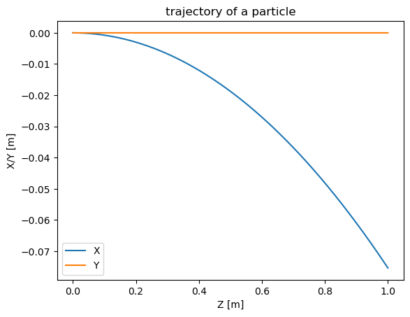
The electron starts with zero transverse coordinates and follows a curved path in the field. The observation point remains (screen.x, screen.y, screen.z) = (0, 0, 1000) m.

warning

For a bunch with a nontrivial phase-space distribution, distinguish the beam-dynamics reference frame from the Cartesian coordinates used by the radiation solver. A practical workflow is to track the bunch to the entrance of the radiating field and then calculate the radiation from those particle coordinates. See Tutorial N9, Simple accelerator-based THz source.

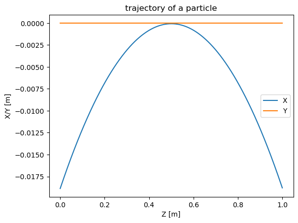
To observe radiation from the central part of the magnet, we modify the electron's initial coordinates. First, determine the required offset.

# the beam momentum 
p = np.sqrt(beam.E**2 - m_e_GeV**2)/speed_of_light

# radius of the trajectory in the bending magnet
R = p*1e9 /By
print("R = ", R, " m")

# angle of the bend
phi = np.arcsin(1 / R)
print("analytical solution: phi = ", phi, " rad")
print("numerical solution: phi ", np.abs(screen.beam_traj.xp(0)[-1]), " rad")

# offset 
x_off = R * (1 - np.cos(phi/2)) 
print("Offset in X direction: ", x_off, " m")

R =  6.671281686212527  m
analytical solution: phi =  0.15046332005984778  rad
numerical solution: phi  0.151609149365928  rad
Offset in X direction:  0.018870166315482287  m

Recalculate radiation with new initial coordinates

beam = Beam()
beam.E = 2            # beam energy in [GeV]
beam.I = 0.1            # beam current in [A]

# set new initial coordinates for the beam
beam.xp = phi/2  # initial angle x'
beam.x = -x_off  # initial offset 


screen = Screen()
screen.z = 1000.0      # distance from the beginning of lattice to the screen

screen.start_energy = 100      # [eV], starting photon energy
screen.end_energy = 20000       # [eV], ending photon energy
screen.num_energy = 500        # number of energy points[eV]


# Calculate radiation 
start = time.time()
screen = calculate_radiation(lat_b, screen, beam, accuracy=6)
print("time exec: ", time.time() - start)

# display trajectory
x = screen.beam_traj.x(0)
y = screen.beam_traj.y(0)
z = screen.beam_traj.z(0)
plt.title("trajectory of a particle")
plt.plot(z, x, label="X")
plt.plot(z, y, label="Y")
plt.xlabel("Z [m]")
plt.ylabel("X/Y [m]")
plt.legend()
plt.show()

# show result
show_flux(screen, unit="mrad",  nfig=204, xlog=False, ylog=False)

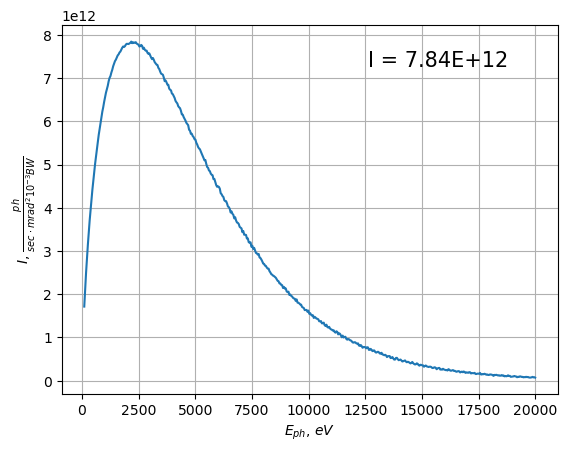
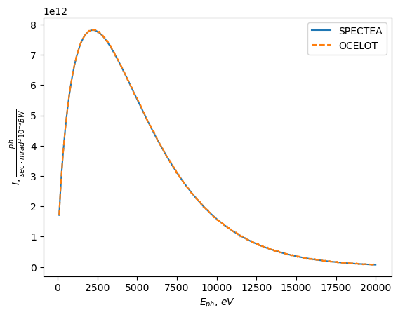
Compare the flux density with SPECTRA

The same setup was simulated with SPECTRA; the result is stored in bm_spectra.dc0.

# load SPECTRA result
a = np.loadtxt("bm_spectra.dc0", skiprows=2, usecols=[0, 1])


plt.plot(a[:,0], a[:,1], label="SPECTRA")
plt.plot(screen.Eph, screen.Total * screen.z**2, "--", label="OCELOT")
plt.ylabel(r"$I$, $\frac{ph}{sec \cdot mrad^2 10^{-3}BW}$")
plt.xlabel(r'$E_{ph}$, $eV$')
plt.legend()
plt.show()