This notebook was created by Andrei Trebushinin (trebandrej@gmail.com) and Svitozar Serkez. August 2019.
2. Coherent radiation module and RadiationField object.
OCELOT has the RadiationField object which represents a 3D electric field distribution, initially in space-time domain
%matplotlib inline
import logging
import ocelot
from ocelot.common.globals import *
from ocelot.optics.wave import RadiationField, dfl_waistscan
from ocelot.optics.wave import imitate_sase_dfl, dfl2wig, dfl_waistscan, generate_gaussian_dfl, dfl_ap_rect, dfl_ap_circ, dfl_interp, wigner_smear, dfl_chirp_freq
from ocelot.gui.dfl_plot import plot_dfl, plot_wigner, plot_dfl_waistscan
from copy import deepcopy
from ocelot import ocelog

ocelog.setLevel(logging.WARNING)
#ocelog.setLevel(logging.DEBUG)
#ocelog.setLevel(logging.INFO)
initializing ocelot...
Contents
- Generating Gaussian RadiationField
- Plotting
- Focusing
- Propagating
- Aperturing
- Interpolating
- Space-frequency analysis
dfl = RadiationField()
help(RadiationField)
    Help on class RadiationField in module ocelot.optics.wave:

    class RadiationField(builtins.object)
     |  RadiationField(shape=(0, 0, 0))
     |
     |  3d or 2d coherent radiation distribution, *.fld variable is the same as Genesis dfl structure
     |
     |  Methods defined here:
     |
     |  E(self)
     |      energy in the pulse [J]
     |
     |  Lx(self)
     |      full transverse horizontal mesh size
     |
     |  Ly(self)
     |      full transverse vertical mesh size
     |
     |  Lz(self)
     |      full longitudinal mesh size
     |
     |  Nstat(self)
     |      number of stat points
     |
     |  Nx(self)
     |      number of points in x
     |
     |  Ny(self)
     |      number of points in y
     |
     |  Nz(self)
     |      number of points in z
     |
     |  __getitem__(self, i)
     |
     |  __init__(self, shape=(0, 0, 0))
     |      Initialize self.  See help(type(self)) for accurate signature.
     |
     |  __setitem__(self, i, fld)
     |
     |  ang_z_onaxis(self)
     |      on-axis phase
     |
     |  coh(self, jit=0)
     |      calculates degree of transverse coherence
     |      consider downsampling the field first
     |
     |  copy_param(self, dfl1, version=1)
     |
     |  curve_wavefront(self, r=inf, plane='xy', domain_z=None)
     |      introduction of the additional
     |      wavefront curvature with radius r
     |
     |      r can be scalar or vector with self.Nz() points
     |      r>0 -> converging wavefront
     |
     |      plane is the plane in which wavefront is curved:
     |          'x' - horizontal focusing
     |          'y' - vertical focusing
     |          'xy' - focusing in both planes
     |
     |      domain_z is the domain in which wavefront curvature is introduced
     |          'f' - frequency
     |          't' - time
     |          None - original domain (default)
     |
     |  disperse(self, disp=0, E_ph0=None, plane='x', return_orig_domains=True)
     |      introducing angular dispersion in given plane by deflecting the radaition by given angle depending on its frequency
     |      disp is the dispertion coefficient [rad/eV]
     |      E_ph0 is the photon energy in [eV] direction of which would not be changed (principal ray)
     |
     |  domains(self)
     |      returns domains of the radiation field
     |
     |  event(self, eventn=0)
     |
     |  fft_xy(self, method='mp', nthread=12, **kwargs)
     |
     |  fft_z(self, method='mp', nthread=12, **kwargs)
     |
     |  fileName(self)
     |
     |  int_x(self)
     |      intensity projection on x
     |
     |  int_xy(self)
     |
     |  int_y(self)
     |      intensity projection on y
     |
     |  int_z(self)
     |      intensity projection on z
     |      power [W] or spectral density [arb.units]
     |
     |  int_zx(self)
     |
     |  int_zy(self)
     |
     |  intensity(self)
     |      3d intensity, abs(fld)**2
     |
     |  mut_coh_func(self, norm=1, jit=1)
     |      calculates mutual coherence function
     |      see Goodman Statistical optics EQs 5.2-7, 5.2-11
     |      (for instance 1985 edition, in 2nd ed. from 2005 equation numbers are different)
     |      returns matrix [y,x,y',x']
     |      consider downsampling the field first
     |
     |  mut_coh_func_c(self, center=(0, 0), norm=1)
     |      Function to calculate mutual coherence function cenetered at xy position
     |
     |      Parameters
     |      ----------
     |      center_xy : tuple, optional
     |          DESCRIPTION.
     |          point with respect to which correlation is calculated
     |          The default is (0,0) (center)
     |          accepts values either in [m] if domain=='s'
     |                             or in [rad] if domain=='k'
     |      norm : TYPE, optional
     |          DESCRIPTION.
     |          The default is 1.
     |          flag of normalization by intensity
     |      Returns
     |      -------
     |      J : TYPE
     |          mutual coherence function matrix [ny, nx]
     |
     |  ph_sp_dens(self)
     |
     |  phen(self)
     |
     |  prop(self, z, fine=1, return_result=0, return_orig_domains=1, **kwargs)
     |      Angular-spectrum propagation for fieldfile
     |
     |      can handle wide spectrum
     |        (every slice in freq.domain is propagated
     |         according to its frequency)
     |      no kx**2+ky**2<<k0**2 limitation
     |
     |      dfl is the RadiationField() object
     |      z is the propagation distance in [m]
     |      fine=1 is a flag for ~2x faster propagation.
     |          no Fourier transform to frequency domain is done
     |          assumes no angular dispersion (true for plain FEL radiation)
     |          assumes narrow spectrum at center of xlamds (true for plain FEL radiation)
     |
     |      return_result does not modify self, but returns result
     |
     |      z>0 -> forward direction
     |
     |  prop_m(self, z, m=1, fine=1, return_result=0, return_orig_domains=1, **kwargs)
     |      Angular-spectrum propagation for fieldfile
     |
     |      can handle wide spectrum
     |        (every slice in freq.domain is propagated
     |         according to its frequency)
     |      no kx**2+ky**2<<k0**2 limitation
     |
     |      dfl is the RadiationField() object
     |      z is the propagation distance in [m]
     |      m is the output mesh size in terms of input mesh size (m = L_out/L_inp)
     |      which can be a number m or a pair of number m = [m_x, m_y]
     |      fine==0 is a flag for ~2x faster propagation.
     |          no Fourier transform to frequency domain is done
     |          assumes no angular dispersion (true for plain FEL radiation)
     |          assumes narrow spectrum at center of xlamds (true for plain FEL radiation)
     |
     |      z>0 -> forward direction
     |
     |  scale_kx(self)
     |      # propper scales in meters or 2 pi / meters
     |
     |  scale_ky(self)
     |
     |  scale_kz(self)
     |
     |  scale_x(self)
     |
     |  scale_y(self)
     |
     |  scale_z(self)
     |
     |  shape(self)
     |      returns the shape of fld attribute
     |
     |  slices2stat(self)
     |
     |  stat2slices(self)
     |
     |  tilt(self, angle=0, plane='x', return_orig_domains=True)
     |      deflects the radaition in given direction by given angle
     |      by introducing transverse phase chirp
     |
     |  to_domain(self, domains='ts', **kwargs)
     |      tranfers radiation to specified domains
     |      *domains is a string with one or two letters:
     |          ("t" or "f") and ("s" or "k")
     |      where
     |          't' (time); 'f' (frequency); 's' (space); 'k' (inverse space);
     |      e.g.
     |          't'; 'f'; 's'; 'k'; 'ts'; 'fs'; 'tk'; 'fk'
     |      order does not matter
     |
     |      **kwargs are passed down to self.fft_z and self.fft_xy
     |
     |  ----------------------------------------------------------------------
     |  Data descriptors defined here:
     |
     |  __dict__
     |      dictionary for instance variables (if defined)
     |
     |  __weakref__
     |      list of weak references to the object (if defined)
Generating Gaussian RadiationField
We will demonstrate capabilities of this object using a model gaussian beam. The 3D gaussian beam radiation pulse can be defined with the following arguments:
help(generate_gaussian_dfl)

E_pohoton = 8000 #central photon energy [eV]
kwargs={'xlamds':(h_eV_s * speed_of_light / E_pohoton), #[m] - central wavelength
        'shape':(301,301,10),           #(x,y,z) shape of field matrix (reversed) to dfl.fld
        'dgrid':(500e-6,500e-6,1e-6), #(x,y,z) [m] - size of field matrix
        'power_rms':(3e-6,10e-6,0.1e-6),#(x,y,z) [m] - rms size of the radiation distribution (gaussian)
        'power_center':(0,0,None),     #(x,y,z) [m] - position of the radiation distribution
        'power_angle':(0,0),           #(x,y) [rad] - angle of further radiation propagation
        'power_waistpos':(-5,-15),     #(Z_x,Z_y) [m] downstrean location of the waist of the beam
        'wavelength':None,             #central frequency of the radiation, if different from xlamds
        'zsep':None,                   #distance between slices in z as zsep*xlamds
        'freq_chirp':0,                #dw/dt=[1/fs**2] - requency chirp of the beam around power_center[2]
        'en_pulse':None,               #total energy or max power of the pulse, use only one
        'power':1e6,
        }
dfl = generate_gaussian_dfl(**kwargs);
    Help on function generate_gaussian_dfl in module ocelot.optics.wave:

    generate_gaussian_dfl(xlamds=1e-09, shape=(51, 51, 100), dgrid=(0.001, 0.001, 5e-05), power_rms=(0.0001, 0.0001, 5e-06), power_center=(0, 0, None), power_angle=(0, 0), power_waistpos=(0, 0), wavelength=None, zsep=None, freq_chirp=0, en_pulse=None, power=1000000.0, **kwargs)
        generates RadiationField object
        narrow-bandwidth, paraxial approximations

        xlamds [m] - central wavelength
        shape (x,y,z) - shape of field matrix (reversed) to dfl.fld
        dgrid (x,y,z) [m] - size of field matrix
        power_rms (x,y,z) [m] - rms size of the radiation distribution (gaussian)
        power_center (x,y,z) [m] - position of the radiation distribution
        power_angle (x,y) [rad] - angle of further radiation propagation
        power_waistpos (x,y) [m] downstrean location of the waist of the beam
        wavelength [m] - central frequency of the radiation, if different from xlamds
        zsep (integer) - distance between slices in z as zsep*xlamds
        freq_chirp dw/dt=[1/fs**2] - requency chirp of the beam around power_center[2]
        en_pulse, power = total energy or max power of the pulse, use only one
The RadiationField object is a 3D data cube in dfl.fld attribute (numpy array) with a dfl.fld.shape = dfl.shape() = (Nz, Nx, Ny) and a grid step for each axis dfl.dx , dfl.dy , dfl.dz so that dgrid[0], dgrid[1], dgrid[2] = dx*Nx, dy*Ny, dz*Nz.
We created the gaussian beam with location of its horizontal waist at -5 meters and vertical waist at -15 meters location (wavefront is divergent now)
Plotting
To visulize the radiation one can use plot_dfl() function. There is an option to plot the radiation in what domain you want (transverse: 's'pace and 'k'-inverse space, longitudinal: 't'ime and 'f'requency) and any combination of them.
help(plot_dfl)

plot_dfl(dfl, #RadiationField() object
         domains=None, #longitudinal domain + transverse domain ('t' or 'f' + 's' or 'k')
                       #(example: 'tk' - time/inversespace domain)
         z_lim=[],     #sets the boundaries to CUT the dfl object in z to ranges of e.g. [2,5] um or nm depending on freq_domain=False of True
         xy_lim=[],    #sets the boundaries to SCALE the dfl object in x and y to ranges of e.g. [2,5] um or urad depending on far_field=False of True
         figsize=4,    #rescales the size of the figure
         cmap='viridis',    #colormap which will be used for plotting (http://matplotlib.org/users/colormaps.html)
         phase=True,   #bool type variable, can replace Z projection or spectrum with phase front distribution z dimensions correspondingly
         fig_name='default_dfl_plot', #the desired name of the output figure, would be used as suffix to the image filename if savefig==True
         auto_zoom=False,  #bool type variable, automatically scales xyz the images to the (1%?) of the intensity limits
         column_3d=True,   #bool type variable, plots top and side views of the radiation distribution
         savefig=False,    #bool type variable, allow to save figure to image (savefig='png' (default) or savefig='eps', etc...)
         showfig=True,     #bool type variable, allow to display figure (slower)
         return_proj=False,#bool type variable, returns [xy_proj,yz_proj,xz_proj,x,y,z] array.
         line_off_xy=True, #bool type variable, if True, the transverse size of radiation are calculated at x=0 and y=0 position, otherwise marginal distributions are provided
         log_scale=0,      #bool type variable, if True, log scale will be used for potting
         cmap_cutoff=0)   #0 <= cmap_cutoff <= 1; all pixels that have intensity lower than cmap_cutoff will be seted to white color
    Help on function plot_dfl in module ocelot.gui.dfl_plot:

    plot_dfl(dfl, domains=None, z_lim=[], xy_lim=[], figsize=4, cmap='viridis', legend=True, phase=False, fig_name=None, auto_zoom=False, column_3d=True, savefig=False, showfig=True, return_proj=False, line_off_xy=True, slice_xy=False, log_scale=0, cmap_cutoff=0, vartype_dfl=None, plot_sp_dens=True, event=None, **kwargs)
        Plots dfl radiation object in 3d using matplotlib.

        :param dfl: RadiationField() object
        :param domains: longitudinal domain + transverse domain ('t' or 'f' + 's' or 'k') (example: 'tk' - time/inversespace domain)
        :param z_lim: sets the boundaries to CUT the dfl object in z to ranges of e.g. [2,5] um or nm depending on freq_domain=False of True
        :param xy_lim: sets the boundaries to SCALE the dfl object in x and y to ranges of e.g. [2,5] um or urad depending on far_field=False of True
        :param figsize: rescales the size of the figure
        :param cmap: color map which will be used for plotting (http://matplotlib.org/users/colormaps.html)
        :param legend: not used yet
        :param phase: bool type variable, can replace Z projection or spectrum with phase front distribution z dimensions correspondingly
        :param fig_name: the desired name of the output figure, would be used as suffix to the image filename if savefig==True
        :param auto_zoom: bool type variable, automatically scales xyz the images to the (1%?) of the intensity limits
        :param column_3d: bool type variable, plots top and side views of the radiation distribution
        :param savefig: bool type variable, allow to save figure to image (savefig='png' (default) or savefig='eps', etc...)
        :param showfig: bool type variable, allow to display figure (slower)
        :param return_proj: bool type variable, returns [xy_proj,yz_proj,xz_proj,x,y,z] array.
        :param line_off_xy: bool type variable, if True, the transverse size of radiation are calculated at x=0 and y=0 position, otherwise marginal distribution are used
        :param slice_xy: bool type variable, if True, slices will be plotted; if False, projections will be plotted
        :param log_scale: bool type variable, if True, log scale will be used for potting
        :param cmap_cutoff: 0 <= cmap_cutoff <= 1; all pixels that have intensity lower than cmap_cutoff will be seted to white color
        :param vartype_dfl: the data type to store dfl in memory [either complex128 (two 64-bit floats) or complex64 (two 32-bit floats)], may save memory (deprecated)
        :param plot_sp_dens: whether to recalculate spectral density in units of mJ/eV
        :param event: allows to choolse which statistical realization (element of dfl.fld_stat=[]) we wish to plot
        :param kwargs:
        :return:
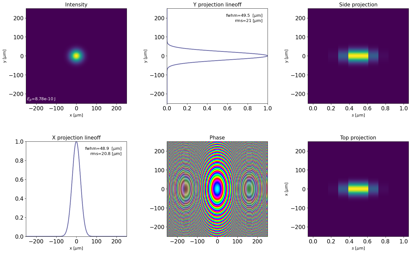
Plotting radiation in inverse space - frequency domain
plot_dfl(dfl, domains='kf')
Focusing
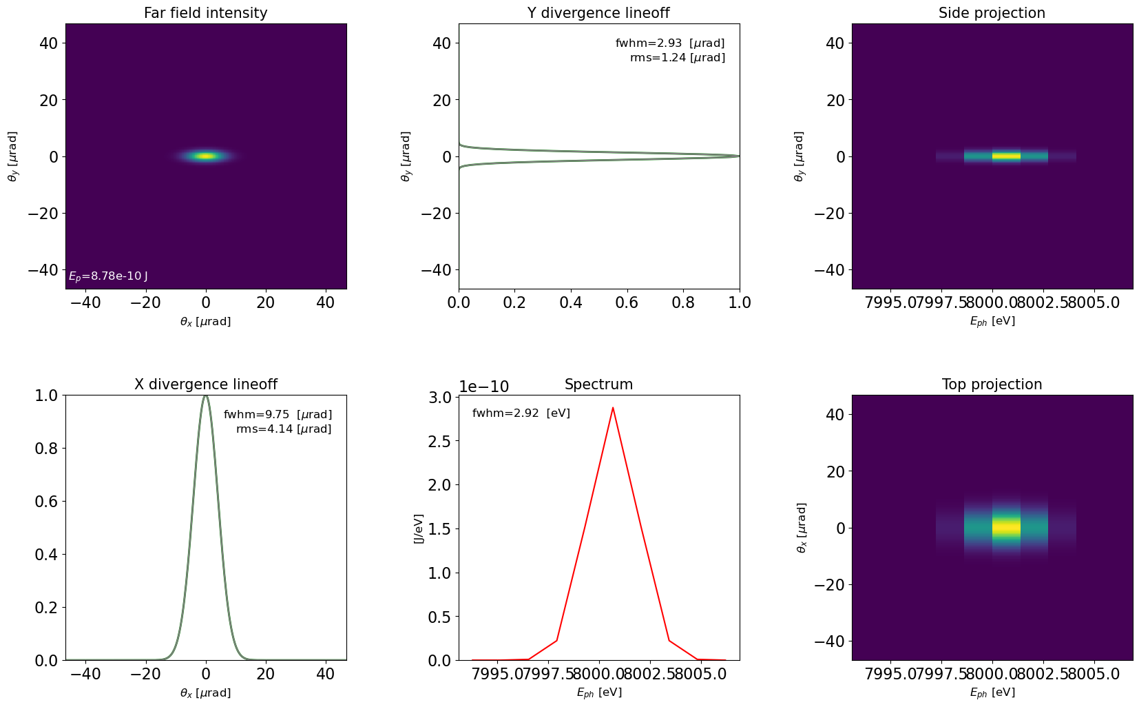
Apply additional curvature to the radiation field wavefront along the given plane: 'x' or 'y' Here we collimate the radiation in 'x' direction. Note the different radius of curvature needed to collimate the beam, compared to the distance from the waist in Gaussian beam.
help(RadiationField().curve_wavefront)

dfl0 = deepcopy(dfl)
plot_dfl(dfl0, column_3d=False, phase=True)
dfl0.curve_wavefront(r=5.1, plane='x')
plot_dfl(dfl0, column_3d=False, phase=True)
    Help on method curve_wavefront in module ocelot.optics.wave:

    curve_wavefront(r=inf, plane='xy', domain_z=None) method of ocelot.optics.wave.RadiationField instance
        introduction of the additional
        wavefront curvature with radius r

        r can be scalar or vector with self.Nz() points
        r>0 -> converging wavefront

        plane is the plane in which wavefront is curved:
            'x' - horizontal focusing
            'y' - vertical focusing
            'xy' - focusing in both planes

        domain_z is the domain in which wavefront curvature is introduced
            'f' - frequency
            't' - time
            None - original domain (default)

Propagating
RadiationField() class has a Fresnel Transfer Function Propagator method RadiationField().prop(z, fine=1, return_result=0, return_orig_domains=1) which calculates the radiation distribution at some distance z with the exact free space response function .
So that the field ad distance would be (see e.g. Voelz, David George. Computational fourier optics: a MATLAB tutorial. Bellingham, WA: SPIE press, 2011)
The method accepts the following parameters:
z- propagation distance [m]; z>0 corresponds to forward directionfineis an accuracy parameter. iffine==0, no Fourier transform to frequency domain is done, allows 2x faster calculation applicable for plain SASE radiation.return_orig_domainsisTrueby default, otherwise, time is spared
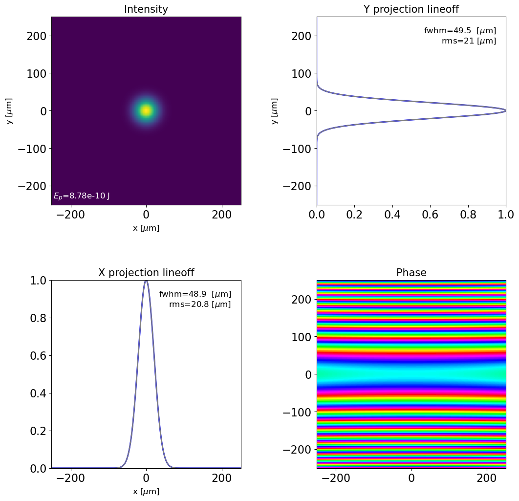
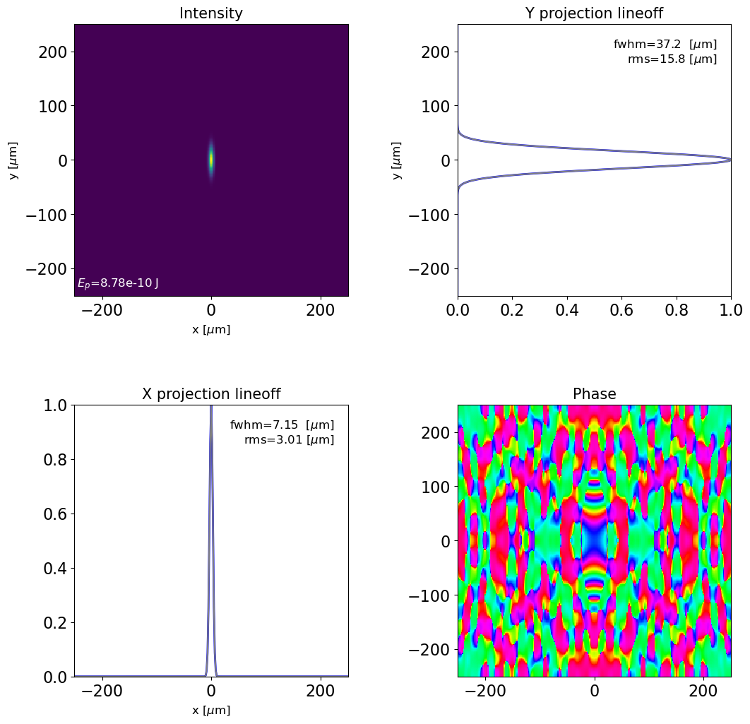
We propagate the field to its horizontal waist.
dfl0 = deepcopy(dfl)
dfl0.prop(z=-5) #propagation distance [m]
plot_dfl(dfl0, fig_name='dfl_prop', phase=True, column_3d=False)
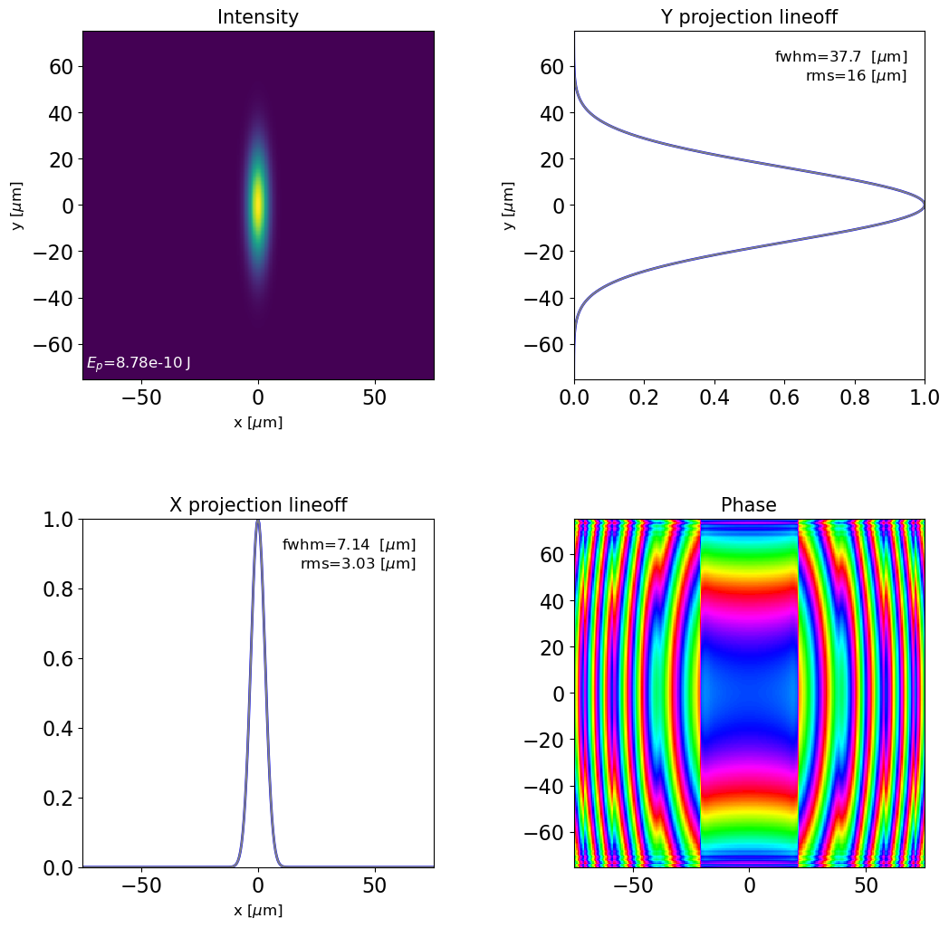
One can change the grid spacing in the resulting plane upon propagation, using Angular-Spectrum Propagation with scaling parameter m, see Schmidt, Jason Daniel. "Numerical simulation of optical wave propagation with examples in MATLAB" Bellingham, Washington, USA: SPIE, 2010. Effectively it is done via manipulation of waverfont curvatures before and after the propagation.
The corresponding method .prop_m(z, m=1, fine=1, return_result=0, return_orig_domains=1) has an additional parameter
m- the output mesh size in terms of input mesh size (m = L_out/L_inp). I can be a single number or a tuplem=(m_x, m_y)to account for asymmetric scaling.
dfl0 = deepcopy(dfl)
dfl0.prop_m(z=-5, #propagation distance [m]
            m=0.3   #mesh resize coefficient
            #m=(0.05,0.3)   #asymmetric resize
            )
plot_dfl(dfl0, fig_name='dfl_prop', phase=True, column_3d=False)
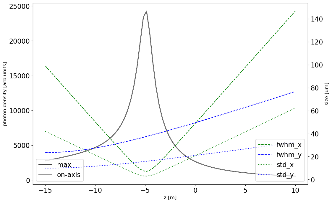
The OCELOT toolkit has a function that scans transverse radiation size (fwhm, std), and power density (on-axis and maximum values) over the defined radiation propogation span with .prop() method. This may allow one to determine e.g. the location of the radiation source inside the undulator.
help(dfl_waistscan)
w_scan = dfl_waistscan(dfl,
                       z_pos=np.linspace(-15,10,80),
                       projection=0)

plot_dfl_waistscan(w_scan,
                   fig_name='waist scan results',
                   showfig=True,
                   savefig=False)
    Help on function dfl_waistscan in module ocelot.optics.wave:

    dfl_waistscan(dfl, z_pos, projection=0, **kwargs)
        propagates the RadaitionField object dfl
        through the sequence of positions z_pos
        and calculates transverse distribution parameters
        such as peak photon density and sizes in both dimensions

        if projection==1, then size of projection is calculated
            otherwise - size across the central line passing through the mesh center
Aperturing
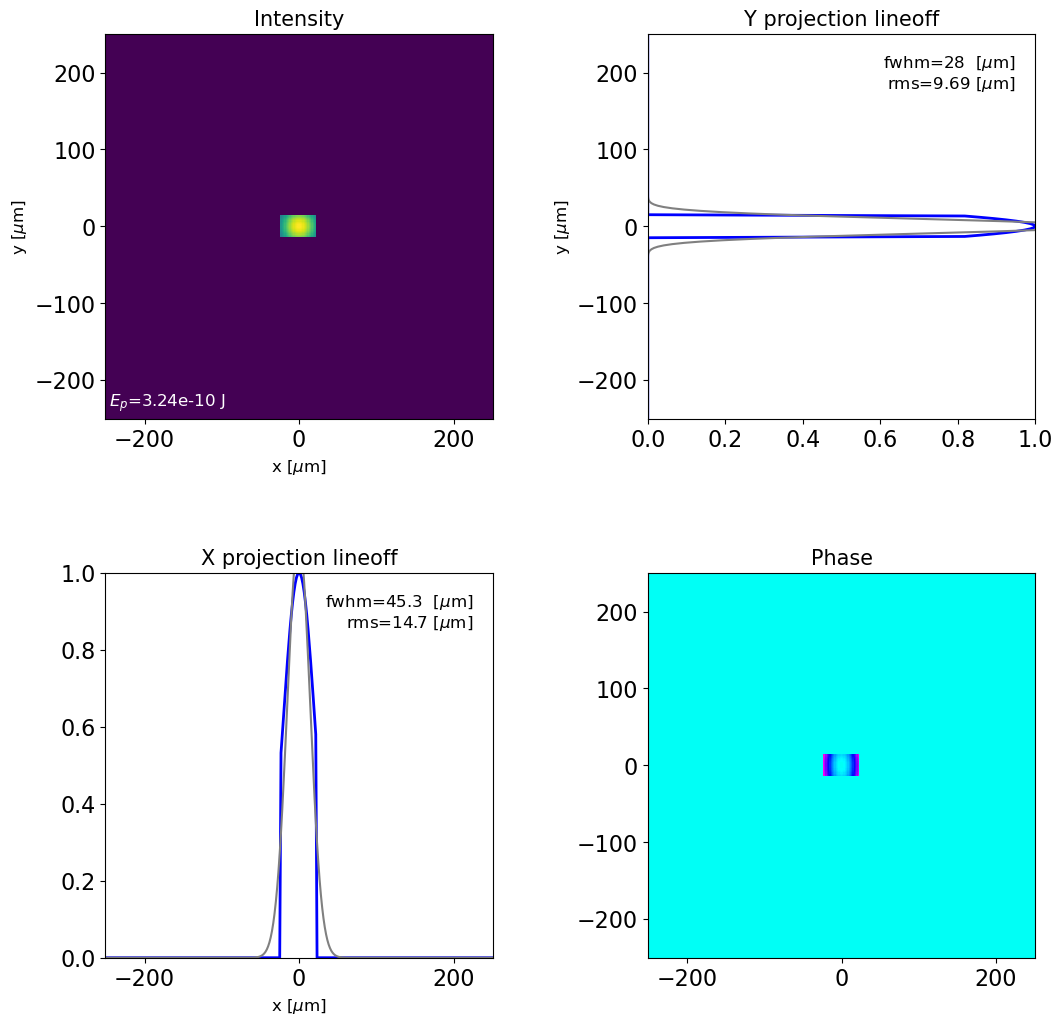
One can introduce a rectangular of a circular aperture and propagate the radiation through it.
dfl0 = deepcopy(dfl)

dfl0 = dfl_ap_rect(dfl0, ap_x=5e-5, ap_y=3e-5) #x and y sizes in [m]
#dfl0 = dfl_ap_circ(dfl0, r=1e-5)

plot_dfl(dfl0, fig_name='dfl_ap', phase=True, column_3d=False)
#dfl0.prop_m(z=150, m=20)
#plot_dfl(dfl0, fig_name='dfl_ap_prop', phase=True, column_3d=False)
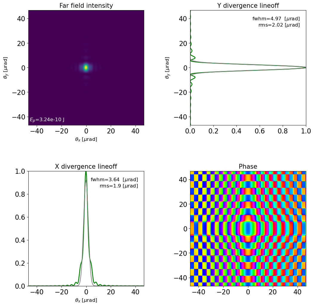
plot_dfl(dfl0, domains = 'kt', fig_name='dfl_ap_prop', phase=True, column_3d=False, log_scale=0)
Interpolating
RaidationField can be interpolated with dfl_interp() function.
When newN and newL are not None, interpN and interpL values are ignored.
Here scipy.interpolate.interp2d method is used
help(dfl_interp)

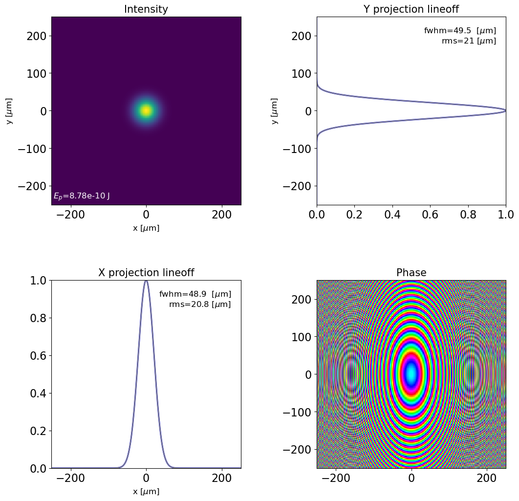
dfl0 = deepcopy(dfl)
print('N_points before interpolation (Nz,Ny,Nx): {:}'.format(dfl0.shape()))
plot_dfl(dfl0, domains = 'st', fig_name='not interpolated', phase=True, column_3d=False)

dfl0 = dfl_interp(dfl0,
                  #interpN=(2, 0.5), #scaling the transverse point density (x,y)
                  #interpL=(1, 1), #scaling the transverse mesh (x,y)
                  newN=(209, 151), #new number of points (x,y)
                  newL=(100e-6, 200e-6), #new mesh size (x,y)
                  method='cubic', #interpolation method
                  return_result=1 #if 0 - mutates the object, if 1 - returns the result
                 )

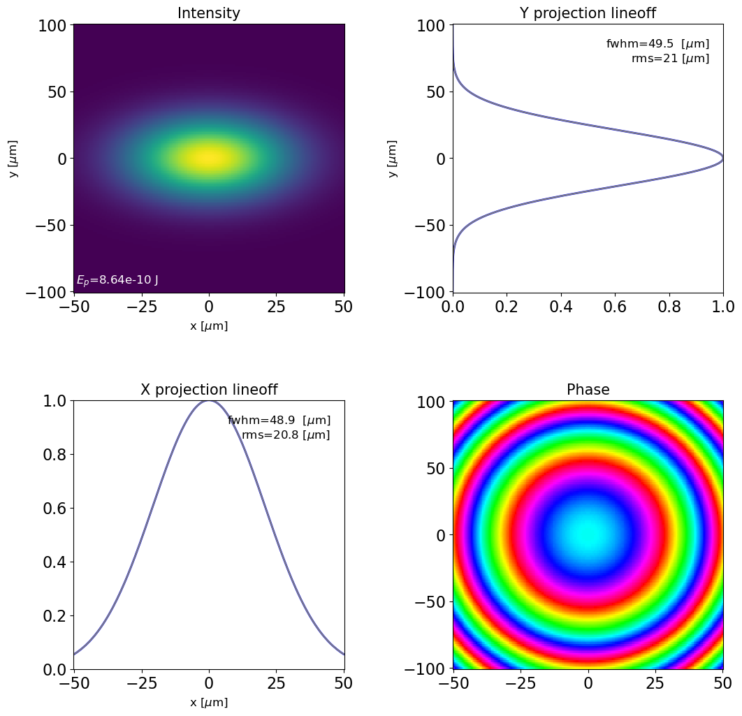
print('N_points after interpolation (Nz,Ny,Nx): {:}'.format(dfl0.shape()))
plot_dfl(dfl0, domains = 'st', fig_name='interpolated', phase=True, column_3d=False)
    Help on function dfl_interp in module ocelot.optics.wave:

    dfl_interp(dfl, interpN=(1, 1), interpL=(1, 1), newN=(None, None), newL=(None, None), method='cubic', return_result=1, **kwargs)
        2d interpolation of the coherent radiation distribution
        interpN and interpL define the desired interpolation coefficients for
        transverse point __density__ and transverse mesh __size__ correspondingly
        newN and newL define the final desire number of points and size of the mesh
        when newN and newL are not None interpN and interpL values are ignored
        coordinate convention is (x,y)

    N_points before interpolation (Nz,Ny,Nx): (10, 301, 301)
N_points after interpolation (Nz,Ny,Nx): (10, 151, 209)
Space-Frequency analysis and manipulation
Calculating on-axis Wigner distribution
let's generate a frequency-chirped radiation field
E_pohoton = 8000 #central photon energy [eV]
kwargs={'xlamds':(h_eV_s * speed_of_light / E_pohoton), #[m] - central wavelength
        'shape':(3,3,1000),           #(x,y,z) shape of field matrix (reversed) to dfl.fld
        'dgrid':(1e-6,1e-6,5e-6), #(x,y,z) [m] - size of field matrix
        'power_rms':(3e-6,3e-6,0.5e-6),#(x,y,z) [m] - rms size of the radiation distribution (gaussian)
        'freq_chirp':0.8,                #dw/dt=[1/fs**2] - requency chirp of the beam around power_center[2]
        }
dfl = generate_gaussian_dfl(**kwargs);  #Gaussian beam defenition
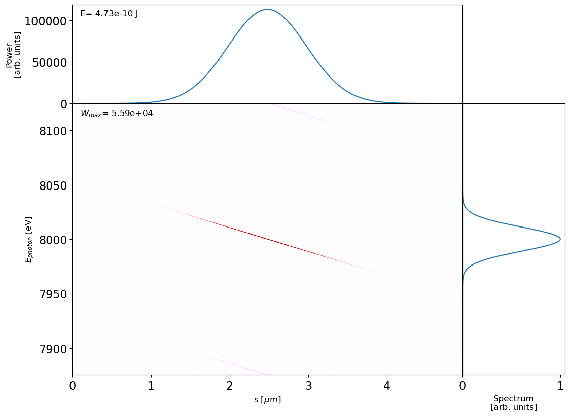
and calculate a Wigner distribution of the on-axis radiation with dfl2wig() function
help(dfl2wig)
wig = dfl2wig(dfl,
                 pad=1 # pads the radiation field values with zeros to increase number of points in <pad> times
                )
    Help on function dfl2wig in module ocelot.optics.wave:

    dfl2wig(dfl, method='mp', pad=1, domain='t', **kwargs)
        returns on-axis WignerDistribution from dfl file
help(plot_wigner)
plot_wigner(wig,
            x_units='um',
            y_units='ev',
            x_lim=(None, None),
            y_lim=(None, None),
            downsample=1,
            autoscale=None,
            figsize=3,
            cmap='seismic',
            fig_name=None,
            savefig=False,
            showfig=True,
            plot_proj=1,
            plot_text=1,
            plot_moments=0,
            plot_cbar=0,
            log_scale=0,
            )
    Help on function plot_wigner in module ocelot.gui.dfl_plot:

    plot_wigner(wig_or_out, *args, **kwargs)
        calls plot_wigner_z or plot_wigner_u depending on domain in the wigner
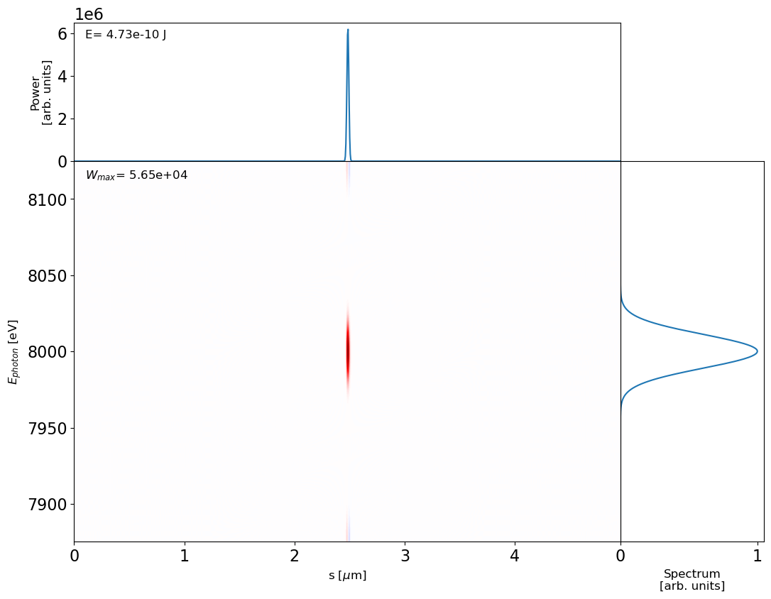
Compress the chirped pulse
help(dfl_chirp_freq)

dfl_ch = dfl_chirp_freq(dfl,
               coeff=(0, 0, 0.099), #coeff[2] is the group delay dispersion (GDD)
               E_ph0=None,
               return_result=True)

plot_wigner(dfl2wig(dfl_ch))
    Help on function dfl_chirp_freq in module ocelot.optics.wave:

    dfl_chirp_freq(dfl, coeff, E_ph0=None, return_result=False)
        The function adds a phase shift to a fld object. The expression for the phase see in the calc_phase_delay function
        dfl   --- is a fld object
        coeff --- coefficients in phase (see in the calc_phase_delay function)
        E_ph0 --- energy with respect to which the phase shift is calculated
        return_result --- a flag that is responsible for returning the modified dfl object if it is True or
                          change the dfl function parameter if it is False
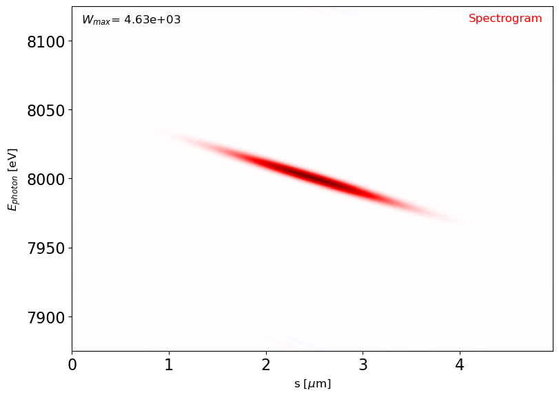
Calculating Spectrogtam
help(wigner_smear)
spectrogram = wigner_smear(wig, sigma_s=0.1e-6)
plot_wigner(spectrogram, figsize=2, plot_proj=0)
    Help on function wigner_smear in module ocelot.optics.wave:

    wigner_smear(wig, sigma_s)
        Convolves wigner distribution with gaussian window function to obtain spectrogram, see https://arxiv.org/pdf/1811.11446.pdf

        :param wig: ocelot.optics.wave.WignerDistribution object which will be convolved with generated window func
        :param sigma_s: [meters] rms size of the s=-ct the gaussian window func
        :return: convolved ocelot.optics.wave.WignerDistribution object with gaussian window function
