This notebook was created by Svitozar Serkez. Source and license info is on GitHub. August 2019.
5. SASE estimation and imitation (unfinished)
%matplotlib inline
import numpy as np
import logging

import ocelot
from ocelot import *
from ocelot.cpbd.beam import *
from ocelot.rad.fel_estimator import *
from ocelot.gui.beam_plot import *
from ocelot.gui.dfl_plot import *

#ocelog.setLevel(logging.ERROR)
#ocelog.setLevel(logging.DEBUG)
ocelog.setLevel(logging.INFO)
plt.clf()
#%matplotlib notebook
    initializing ocelot...
    <Figure size 640x480 with 0 Axes>
Contents
SASE estimator
Knowing the electron beam parameters and the magnetic lattice one can estimate the average SASE power at saturation As the electron beam is typically much longer than the cooperation length, one can slice it into regions that would never interact with each other and estimate power growth in each of those regions with MXie (default) M. Xie, “Exact and variational solutions of 3D eigenmodes in high gain FELs,” Nucl. Instruments Methods Phys. Res. Sect. A Accel. Spectrometers, Detect. Assoc. Equip., vol. 445, no. 1–3, pp. 59–66, 2000 or SSY (assumes optimum beta in each slice) E. L. Saldin, E. A. Schneidmiller, and M. V. Yurkov, “Design formulas for short-wavelength FELs,” Opt. Commun., vol. 235, no. 4–6, pp. 415–420, May 2004 estimations
First, let us generate the beam and lattice objects
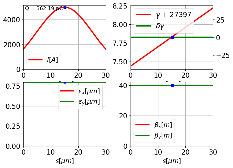
beam = generate_beam(E=14.0, dE=4e-3, I=5000, l_beam=10e-6, emit_n=0.8e-6, beta=40, l_window=30e-6, shape='gaussian', chirp=0.0001)
plot_beam(beam, figsize=2)
[INFO ] [0mgenerating electron beam distribution[0m
[INFO ] : [0mplotting beam[0m
#lat_pkg = create_fel_beamline('EuXFEL_SASE1')
lat_pkg = create_fel_lattice(
                    und_N = 35,
                    und_L = 5,
                    und_l = 0.04,
                    und_Kx = 0,
                    und_Ky = 0,
                    inters_L = 1.08,
                    inters_K = 'K_und',
                    inters_phi=0,
                    quad_L = 0.4,
                    quad_K = 0,
                    phs_L = 0.0,
                    quad_start = 'd')

E_photon=8000
beta_av=20
prepare_el_optics(beam, lat_pkg, E_photon, beta_av, s=None)
lat = lat_pkg[0]

#tws0 = Twiss(beam.pk())
#tws = twiss(lat, tws0=tws0)
#plot_opt_func(lat, tws, top_plot=["E"], legend=False)
#plt.show()
There are several ways to estimate SASE power growth
#fel = beam2fel(beam, lu=0.04, K_peak=3, iwityp=0)
fel = beamlat2fel(beam, lat, smear_m=None, method='mxie', qf=0) #slower, propagates the beam through the magnettic lattice to estimate average beta of poorly matched slices
#fel = parraylat2fel(parray, lat, step=1e-7) # would convert parray to beam and execute beamlat2fel
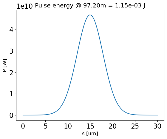
print('zsat = {:.2f}'.format(fel.z_sat_min))
print('E_pulse_sat = {:.2f} uJ'.format(fel.E() * 1e6))
[INFO ] [0mestimating fel from beam and lat[0m
zsat = 79.94
E_pulse_sat = 1145.56 uJ
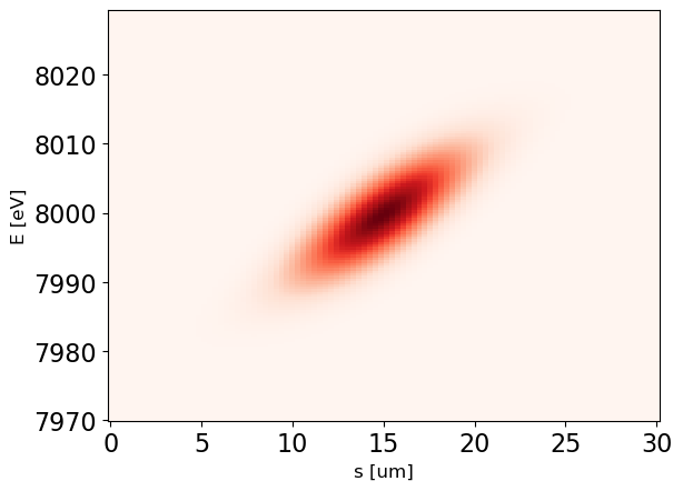
Results can be plotted using the following functions
#fel.log('print')
plot_estimator_power_z(fel, und_duty_factor=5/6.08)
plot_estimator_spectrogram(fel)
plot_estimator_spectrum(fel)
plot_estimator_power_evo(fel, und_duty_factor=5/6.08)
plot_estimator_energy_evo(fel, und_duty_factor=5/6.08)
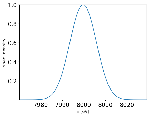
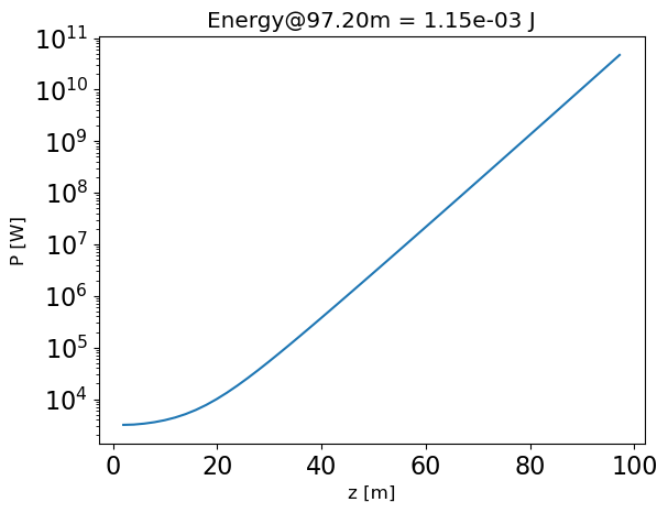
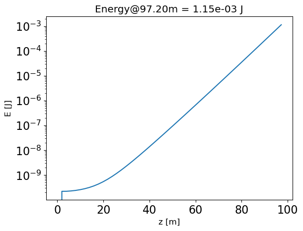

np.trapz(fel.P_sn, fel.s / speed_of_light)
1.8487665968771016e-10
SASE imitator
One can imitate SASE by simulating Gaussian noise and multiplying it by power profile and spectrum profile envelopes in the time and frequency domains respectively, see T. Pfeifer et al. “Partial-coherence method to model experimental free-electron laser pulse statistics”. In: Opt. Lett. 35.20 (2010), p. 3441
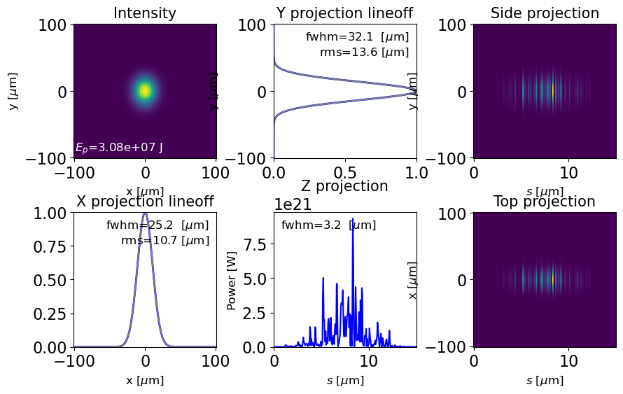
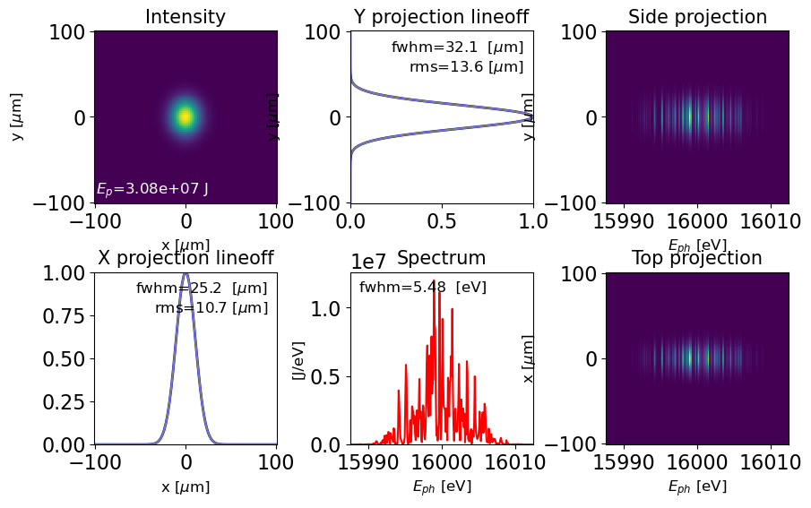
The imitate_sase_dfl function will yield RadiationField object, based on generate_gaussian_dfl, except longitudinally both the amplitudes and phases are modified to yield SASE like spectrum and power. Therefore only the spectral properties of SASE radiation are imitated, while transverse distribution is gaussian, which strictly speaking is not the case.
help(imitate_sase_dfl)

E_pohoton = 16000 #central photon energy [eV]
kwargs={'xlamds':(h_eV_s * speed_of_light / E_pohoton), #[m] - central wavelength
        'shape':(101,101,300),           #(x,y,z) shape of field matrix (reversed) to dfl.fld
        'dgrid':(200e-6,200e-6,15e-6), #(x,y,z) [m] - size of field matrix
        'power_rms':(3e-6,10e-6,2e-6),#(x,y,z) [m] - rms size of the radiation distribution (gaussian)
        'power_center':(0,0,None),     #(x,y,z) [m] - position of the radiation distribution
        'power_angle':(0,0),           #(x,y) [rad] - angle of further radiation propagation
        'power_waistpos':(-5,-15),     #(Z_x,Z_y) [m] downstrean location of the waist of the beam
        'wavelength':None,             #central frequency of the radiation, if different from xlamds
        'zsep':None,                   #distance between slices in z as zsep*xlamds
        'freq_chirp':0,                #dw/dt=[1/fs**2] - requency chirp of the beam around power_center[2]
        #'en_pulse':1e-6,               #total energy or max power of the pulse, use only one
        'power':1e8,
        'rho':1e-4
        }
dfl = imitate_sase_dfl(**kwargs);
[INFO ] [0mimitating SASE radiation[0m
[INFO ] : [0mgenerating radiation field of shape (nz,ny,nx): (101, 101, 300)[0m
[INFO ] : [0mgenerating 1d radiation field imitating SASE[0m
Help on function imitate_sase_dfl in module ocelot.optics.wave:
imitate_sase_dfl(xlamds, rho=0.0002, seed=None, **kwargs)
imitation of SASE radiation in 3D
xlamds - wavelength of the substracted fast-varying component
rho - half of the expected FEL bandwidth
**kwargs identical to generate_dfl()
returns RadiationField object
plot_dfl(dfl, domains = 'st', figsize=2)
plot_dfl(dfl, domains = 'sf', figsize=2)
[INFO ] : [0mplotting radiation field (dfl)[0m
[INFO ] : [0m: domains=st[0m
[INFO ] : [0mplotting radiation field (dfl)[0m
[INFO ] : [0m: domains=sf[0m
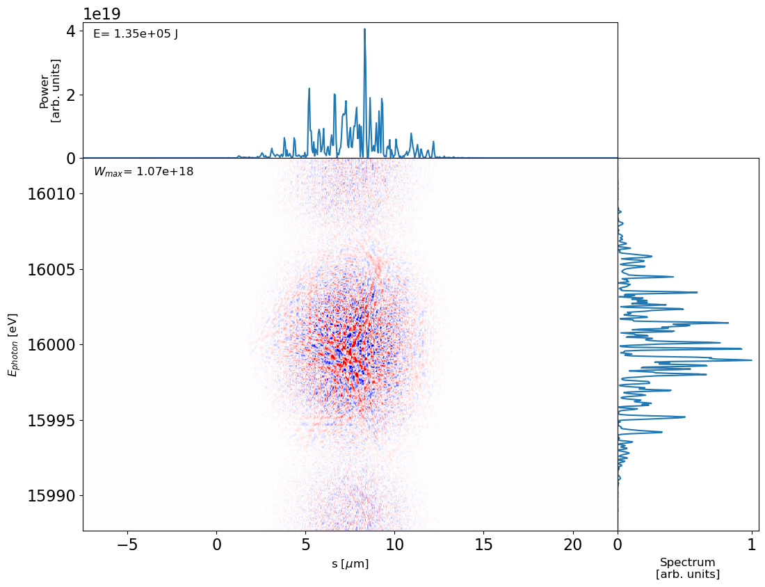
We can study longitudinal Wigner distribution of this SASE-like radiation. extensively discussed in https://journals.iucr.org/s/issues/2021/01/00/co5148/
plot_wigner(dfl2wig(dfl, pad=2))
[INFO ] [0mcalculating Wigner distribution from dfl (on-axis fillament)[0m
[INFO ] : [0mevaluating wigner distribution from 1 event(s)[0m
[INFO ] : : [0mplotting Wigner distribution[0m
