This notebook was created by Mykola Veremchuk (mykola.veremchuk@xfel.eu), Svitozar Serkez. Source and license info is on GitHub. June 2019.

4. Converting synchrotron radiation results from `Screen` object to `RadiationField`

ocelot.optics.wave.RadiationField objects can be used for analysis as well as propagation of Synchrotron radiation module output

2D synchrotron radiation field
3D synchrotron radiation field

Necessary imports

import numpy as np
import logging
from ocelot import *
from ocelot.rad import *
from ocelot.optics.wave import dfl_waistscan, screen2dfl, RadiationField, WignerDistribution, dfl2wig
from ocelot.gui.dfl_plot import plot_dfl, plot_dfl_waistscan, plot_wigner
from ocelot import ocelog

ocelog.setLevel(logging.ERROR) #suppress logger output

    initializing ocelot...

# Activate interactive matplolib in notebook
import matplotlib
%matplotlib inline
# Setup figure white background 
matplotlib.rcParams["figure.facecolor"] = (1,1,1,1)
# Setup figure size
matplotlib.rcParams['figure.figsize'] = [10, 10]

2D synchrotron radiation field

Generating 2D Screen

See PFS tutorial N1. Synchrotron radiation module tutorial first, reproducing the 2d visualization

# generating 2D synchrotron radiation (it will take about 1-3 minutes)
und = Undulator(Kx=0.43, nperiods=500, lperiod=0.007, eid="und")
lat = MagneticLattice(und)

beam = Beam()
beam.E = 2.5  # beam energy in [GeV]
beam.I = 0.1  # beam current in [A]


screen_2d = Screen()
screen_2d.z = 100.0        # distance from the begining of lattice to the screen 
screen_2d.size_x = 0.002   # half of screen size in [m] in horizontal plane
screen_2d.size_y = 0.002   # half of screen size in [m] in vertical plane
screen_2d.nx = 51          # number of points in horizontal plane 
screen_2d.ny = 51          # number of points in vertical plane 


screen_2d.start_energy = 7761.2 # [eV], starting photon energy
screen_2d.end_energy = 7761.2     # [eV], ending photon energy
screen_2d.num_energy = 1        # number of energy points[eV]

screen_2d = calculate_radiation(lat, screen_2d, beam)

Converting 2D Screen to 2D RadiationField

to convert SR from Screen to RadiationField there is a function:

dfl = screen2dfl(screen, polarization='x')

screen: Screen object, electric field of which will be used to generate RadiationField
polarization: polarization for conversion to RadiationField ( $E_x$ or $E_y$ )

see PFS tutorial N2. Coherent radiation module and RadiationField object

dfl_2d = screen2dfl(screen_2d, polarization='x') 

Plotting RadiationField

2D (monochromatic) RadiationFied generated from Screen

plot_dfl(dfl_2d,
         fig_name='dfl_2d generated from screen_2d', 
         column_3d=1)

png

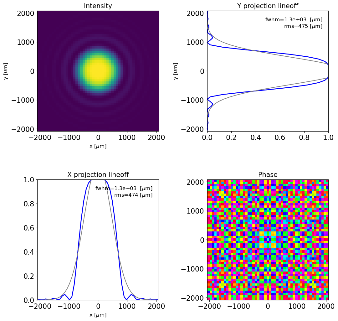
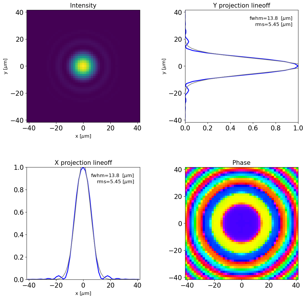
The phase is oscillating very rapidly. Let's study the radiation back-propagated to the middle of the undulator

dfl_2d.prop_m(-100-3.5/2, m=0.02)
plot_dfl(dfl_2d,
         fig_name='dfl_2d generated from screen_2d')

png

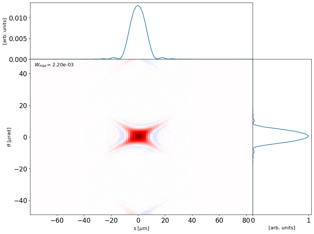
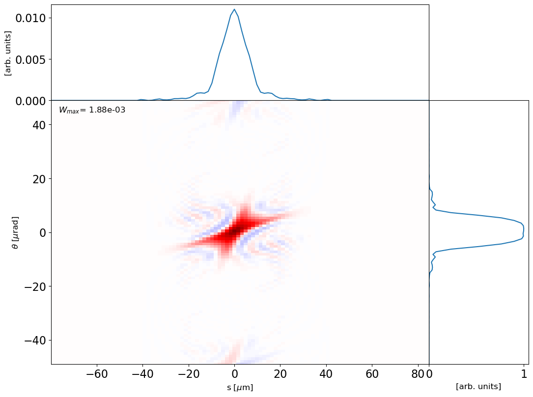
and now we can study transverse Wigner distribution of undulator radiation: (see https://link.aps.org/doi/10.1103/PhysRevSTAB.15.050703 for reference) as the radiation propagates, is evolves, just like the transverse phase-space of an electron beam

wig = dfl2wig(dfl_2d, domain='x', pad=2)
plot_wigner(wig)

plot_wigner(dfl2wig(dfl_2d.prop_m(1, m=1, return_result=True), domain='x', pad=2)) #1m downstream the waist
plot_wigner(dfl2wig(dfl_2d.prop_m(2, m=1, return_result=True), domain='x', pad=2)) #2m downstream the waist

png

Generating and converting 3D Screen

One can calculate series of 2D radiation field distributions at different photon energies.

# generating 3D synchrotron radiation (it will take up to 5 minutes as 75*75*20=112k datapoints are calculated)
screen_3d = Screen()
screen_3d.z = 100.0  # distance from the begining of lattice to the screen
screen_3d.size_x = 0.002  # half of screen size in [m] in horizontal plane
screen_3d.size_y = 0.002  # half of screen size in [m] in vertical plane

screen_3d.ny = 50
screen_3d.nx = 50
screen_3d.start_energy = 7720  # [eV], starting photon energy
screen_3d.end_energy = 7790  # [eV], ending photon energy
screen_3d.num_energy = 25  # number of energy points[eV]

screen_3d = calculate_radiation(lat, screen_3d, beam)
dfl_3d = screen2dfl(screen_3d, polarization='x')

    SR 3D calculation

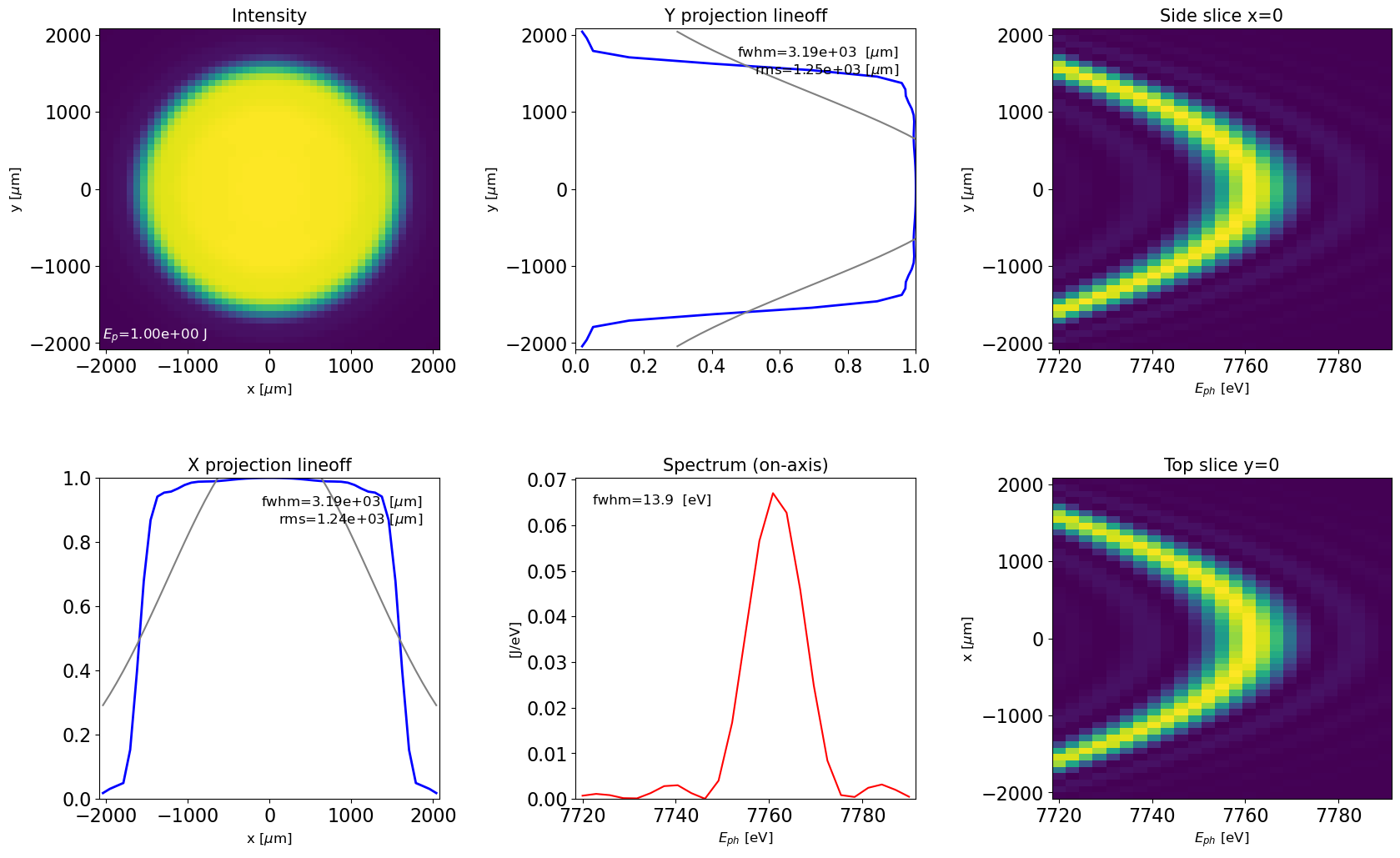
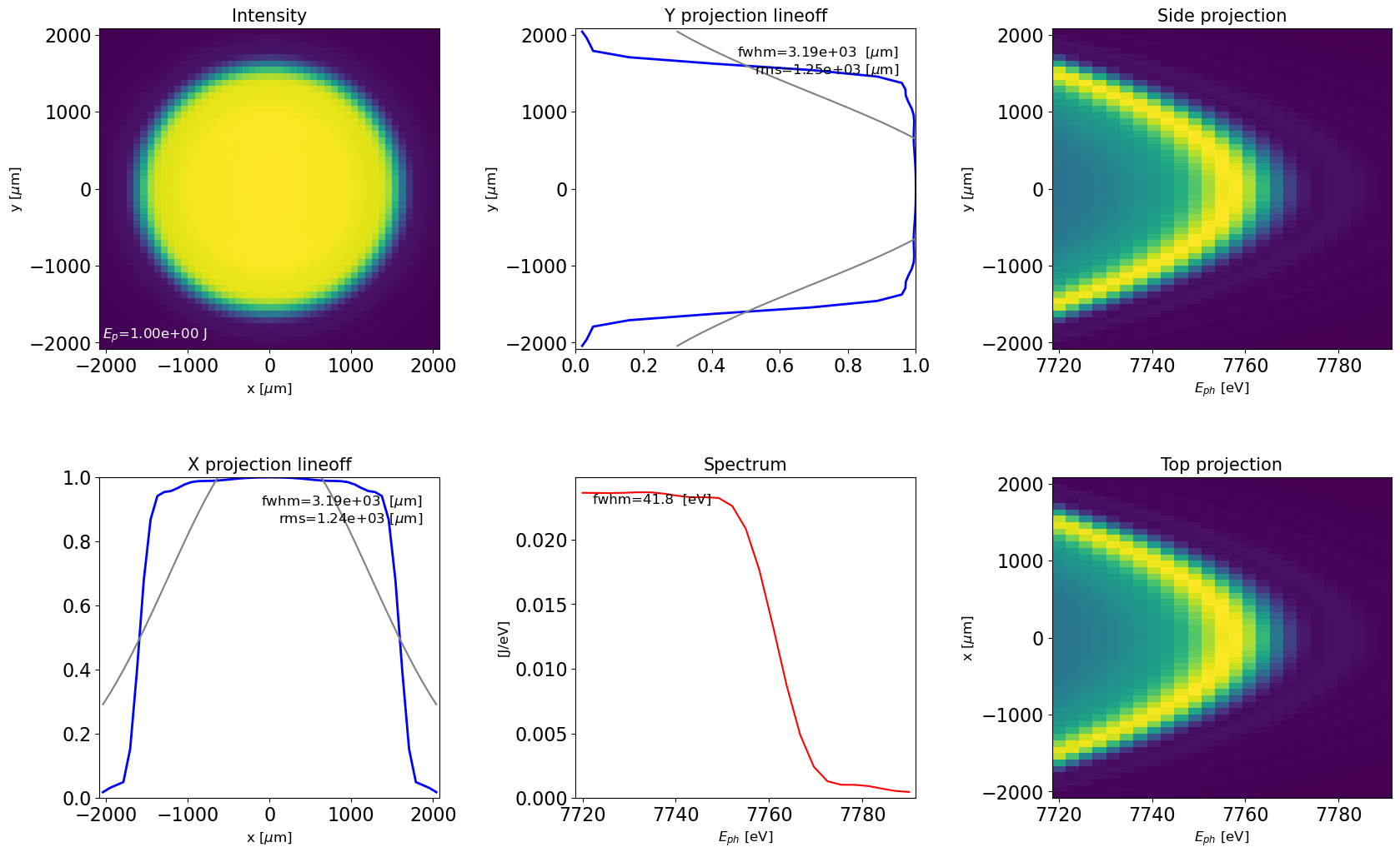
In this way we obtain a 3D RadiationFied distribution in space-frequency domain

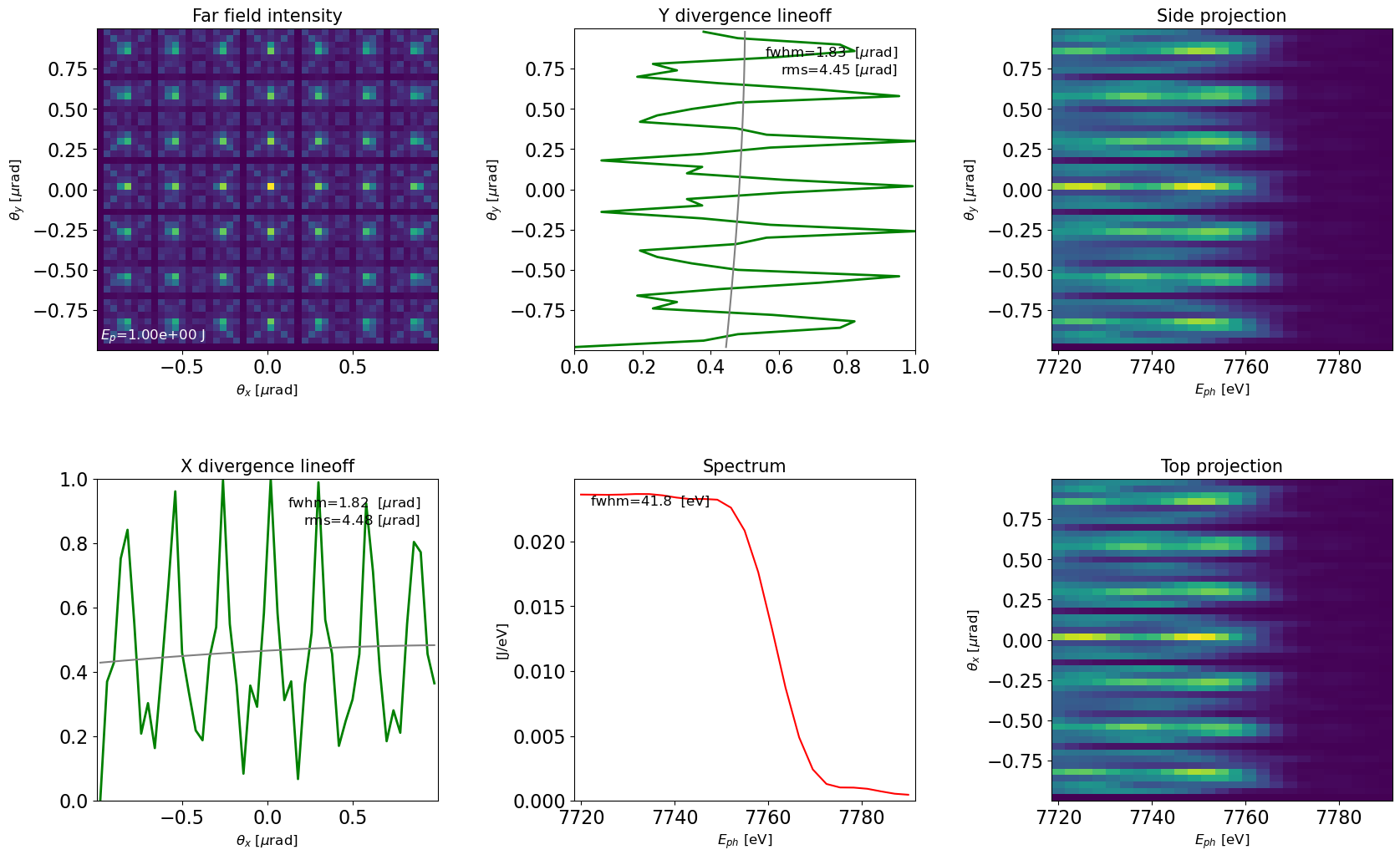
Note the spatial dependence on the photon energy. The slice values of x=0 and y=0 are provided as well as on-axis spectrum

plot_dfl(dfl_3d, 
         domains='sf',
         fig_name='dfl_3d in space-frequency domain',
         slice_xy=True) # bool type variable, if True, slices will be plotted; if False, projections will be plotted

png

Transverse projections and integrated spectrum

plot_dfl(dfl_3d, 
         domains='sf',
         fig_name='dfl_3d in space-frequency domain',
         slice_xy=False)

png

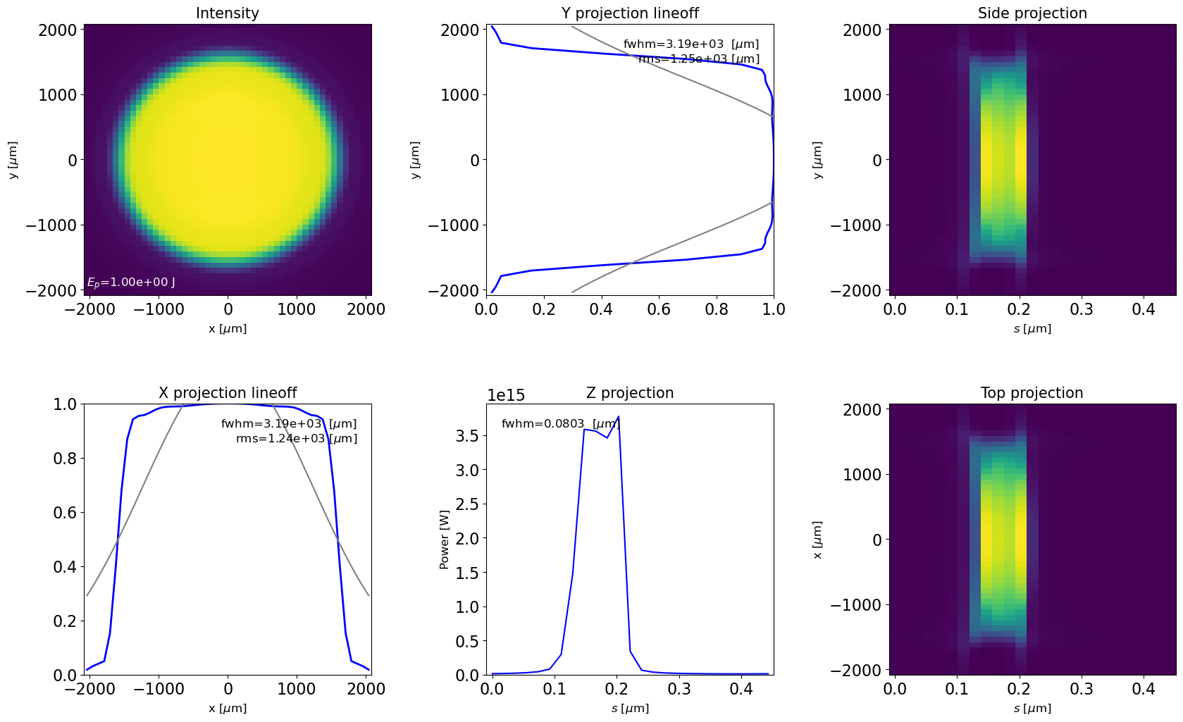
Plotting in space-time domain yields pulse duration that is approximately the radiation wavelength (fundamental harmonic) times number of undulator periods The expected pulse duration from a single electron at this harmonic should be about 0.08um.

plot_dfl(dfl_3d,
         domains='st',
         fig_name='dfl_3d in space-time domain',
         slice_xy=False)

png

Radiation distribution in the middle of the undulator

plot_dfl(dfl_3d.prop_m(-100-3.5/2, m=0.02, fine=1, return_result=1),
         domains='fs',
         fig_name='dfl_3d at waist position in frequency-space domains',
         slice_xy=False)

png

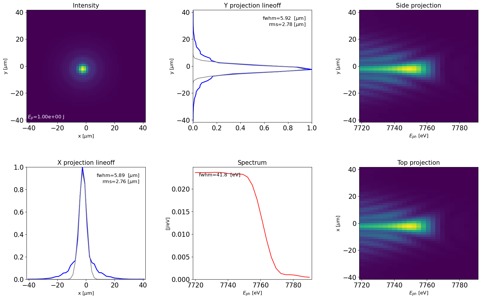
Because of the rapidly-oscilalting phase, plotting in the far zone in not possible yet, to be solved in the future by subtracting spherical phase component

plot_dfl(dfl_3d,
         domains='fk',
         fig_name='dfl_3d at waist position in inverse space-frequency domains',
         slice_xy=False)

png

Contents​

Necessary imports​

2D synchrotron radiation field​

Generating 2D Screen​

Converting 2D Screen to 2D RadiationField​

Plotting RadiationField​

Generating and converting 3D Screen​

Contents