This notebook was created by Sergey Tomin (sergey.tomin@desy.de). Source and license info is on GitHub. January 2018.
Double Bend Achromat
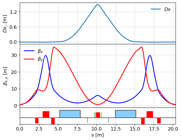
We designed a simple lattice to demonstrate the basic concepts and syntax of the optics functions calculation. Also, we chose DBA to demonstrate the periodic solution for the optical functions calculation.
from __future__ import print_function

# the output of plotting commands is displayed inline within frontends,
# directly below the code cell that produced it
%matplotlib inline

# import from Ocelot main modules and functions
from ocelot import *

# import from Ocelot graphical modules
from ocelot.gui.accelerator import *
Creating lattice
Ocelot has following elements: Drift, Quadrupole, Sextupole, Octupole, Bend, SBend, RBend, Edge, Multipole, Hcor, Vcor, Solenoid, Cavity, Monitor, Marker, Undulator.
# defining of the drifts
D1 = Drift(l=2.)
D2 = Drift(l=0.6)
D3 = Drift(l=0.3)
D4 = Drift(l=0.7)
D5 = Drift(l=0.9)
D6 = Drift(l=0.2)

# defining of the quads
Q1 = Quadrupole(l=0.4, k1=-1.3)
Q2 = Quadrupole(l=0.8, k1=1.4)
Q3 = Quadrupole(l=0.4, k1=-1.7)
Q4 = Quadrupole(l=0.5, k1=1.3)

# defining of the bending magnet
B = Bend(l=2.7, k1=-.06, angle=2*pi/16., e1=pi/16., e2=pi/16.)

# defining of the sextupoles
SF = Sextupole(l=0.01, k2=1.5) #random value
SD = Sextupole(l=0.01, k2=-1.5) #random value

# cell creating
cell = (D1, Q1, D2, Q2, D3, Q3, D4, B, D5, SD, D5, SF, D6, Q4, D6,
        SF, D5, SD, D5, B, D4, Q3, D3, Q2, D2, Q1, D1)
cell
    (<Drift: name=ID_41638795_ at 0x2815f6aa0>,
     <Quadrupole: name=ID_48212357_ at 0x2815f5d50>,
     <Drift: name=ID_92167354_ at 0x2815f6260>,
     <Quadrupole: name=ID_62144763_ at 0x2815f5de0>,
     <Drift: name=ID_65974384_ at 0x2815f69e0>,
     <Quadrupole: name=ID_10916876_ at 0x2815f5db0>,
     <Drift: name=ID_95483235_ at 0x2815f4850>,
     <Bend: name=ID_90868229_ at 0x2815f5f60>,
     <Drift: name=ID_55934688_ at 0x2815f4ac0>,
     <Sextupole: name=ID_22464080_ at 0x11818fee0>,
     <Drift: name=ID_55934688_ at 0x2815f4ac0>,
     <Sextupole: name=ID_30803941_ at 0x2815f5ff0>,
     <Drift: name=ID_49578218_ at 0x2815f4eb0>,
     <Quadrupole: name=ID_27836471_ at 0x2815f5ed0>,
     <Drift: name=ID_49578218_ at 0x2815f4eb0>,
     <Sextupole: name=ID_30803941_ at 0x2815f5ff0>,
     <Drift: name=ID_55934688_ at 0x2815f4ac0>,
     <Sextupole: name=ID_22464080_ at 0x11818fee0>,
     <Drift: name=ID_55934688_ at 0x2815f4ac0>,
     <Bend: name=ID_90868229_ at 0x2815f5f60>,
     <Drift: name=ID_95483235_ at 0x2815f4850>,
     <Quadrupole: name=ID_10916876_ at 0x2815f5db0>,
     <Drift: name=ID_65974384_ at 0x2815f69e0>,
     <Quadrupole: name=ID_62144763_ at 0x2815f5de0>,
     <Drift: name=ID_92167354_ at 0x2815f6260>,
     <Quadrupole: name=ID_48212357_ at 0x2815f5d50>,
     <Drift: name=ID_41638795_ at 0x2815f6aa0>)
*hint: to see a simple description of the function put cursor inside () and press Shift-Tab or you can type sign ? before function. To extend dialog window press + *
Also, one can get more info about element just using print(element)
# all infro about an element can be seen with
print(B)
    Bend(l=2.70000, angle=3.926991e-01, e1=1.963495e-01, e2=1.963495e-01, eid="ID_90868229_")
The cell is a list of the simple objects which contain a physical information of lattice elements such as length, strength, voltage and so on. In order to create a transport map for every element and bind it with lattice object we have to create new Ocelot object - MagneticLattice() which makes these things automatically.
MagneticLattice(sequence, start=None, stop=None, method={"global": TransferMap}):
- sequence - list of the elements,
other parameters we will consider in tutorial N2.
Note, in the current version of OCELOT, transfer map belongs to element. See example# R matrix can be printed for any particular element.
print(Q1.R(energy=0))
    [array([[ 1.10581521,  0.4140116 ,  0.        ,  0.        ,  0.        ,
             0.        ],
           [ 0.53821508,  1.10581521,  0.        ,  0.        ,  0.        ,
             0.        ],
           [ 0.        ,  0.        ,  0.89779021,  0.38627683,  0.        ,
             0.        ],
           [ 0.        ,  0.        , -0.50215988,  0.89779021,  0.        ,
             0.        ],
           [ 0.        ,  0.        ,  0.        ,  0.        ,  1.        ,
             0.        ],
           [ 0.        ,  0.        ,  0.        ,  0.        ,  0.        ,
             1.        ]])]
# or you can directly get transfer maps
Q2.tms
[<ocelot.cpbd.transformations.transfer_map.TransferMap at 0x2815f5ea0>]
lat = MagneticLattice(cell)

# to see total length of the lattice
print("length of the cell: ", lat.totalLen, "m")

# or, for example, you can get R matrix for whole lattice

B, R, T = lat.transfer_maps(energy=0)
print(R)

    length of the cell:  20.34 m
    [[ 0.68401288  0.38454837  0.          0.          0.          0.05268746]
     [-1.38376969  0.68401288  0.          0.          0.          0.23072876]
     [ 0.          0.          0.81775255 -0.29733817  0.          0.        ]
     [ 0.          0.          1.11415489  0.81775255  0.          0.        ]
     [ 0.23072876  0.05268746  0.          0.          1.          0.02228572]
     [ 0.          0.          0.          0.          0.          1.        ]]
Optical function calculation
Uses:
- twiss() function and,
- Twiss() object contains Twiss parameters and other information at one certain position (s) of lattice
To calculate Twiss parameters you have to run twiss(lattice, tws0=None, nPoints=None) function. If you want to get a periodic solution leave tws0 by default.
You can change the number of points over the cell, If nPoints=None, then Twiss parameters are calculated at the end of each element. twiss() function returns list of Twiss() objects.
You will see the Twiss object contains more information than just Twiss parameters.
tws = twiss(lat, nPoints=1000)

# to see Twiss parameters at the beginning of the cell, uncomment next line
# print(tws[0])
print("length = ", len(tws))
# to see Twiss parameters at the end of the cell, uncomment next line
print(tws[-1])
    length =  1000
    emit_x  = 0.0
    emit_y  = 0.0
    beta_x  = 0.5271613695963895
    beta_y  = 0.5165977895295946
    alpha_x = -4.440892098500626e-16
    alpha_y = 6.661338147750939e-15
    gamma_x = 1.8969523521149319
    gamma_y = 1.9357419258618653
    Dx      = 0.16673927708143915
    Dy      = 0.0
    Dxp     = 4.440892098500626e-16
    Dyp     = 0.0
    mux     = 7.100731992120578
    muy     = 5.669884351617213
    nu_x    = 1.1301165961167512
    nu_y    = 0.9023901213192655
    E       = 0.0
    s        = 20.34
# plot optical functions.
plot_opt_func(lat, tws, top_plot = ["Dx", "Dy"], legend=False, font_size=10)
plt.show()

# you also can use standard matplotlib functions for plotting
#s = [tw.s for tw in tws]
#bx = [tw.beta_x for tw in tws]
#plt.plot(s, bx)
#plt.show()

# you can play with quadrupole strength and try to make achromat
Q4.k1 = 1.18

# to make achromat uncomment next line
# Q4.k1 =  1.18543769836
# To use matching function, please see ocelot/demos/ebeam/dba.py

# updating transfer maps after changing element parameters.
#lat.update_transfer_maps() - not needed anymore

# recalculate twiss parameters. Argument nPoints is None by default - Twiss is calculating at the end of each element.
# If you want smooth twiss functions you can set number of points.
tws=twiss(lat, nPoints=1000)

plot_opt_func(lat, tws, legend=False)
plt.show()

More about periodic solution for the Twiss function
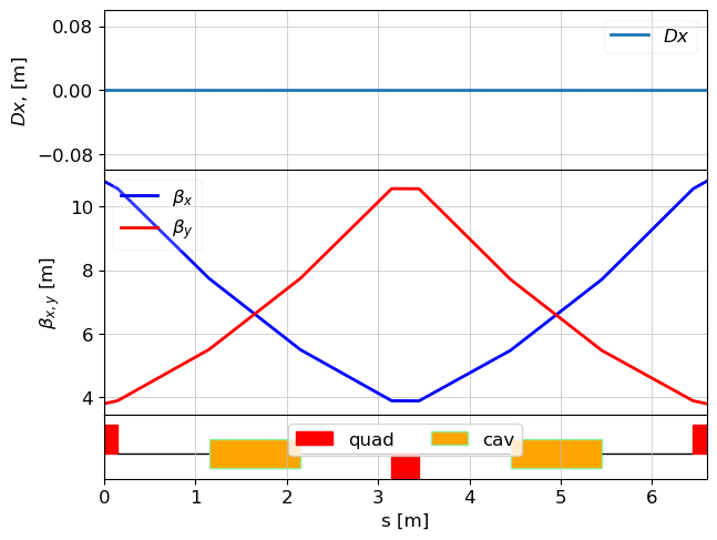
In some cases, one needs to quickly find a periodic solution. Here is a simple example with Cavity element:
d = Drift(l=1)
qf_h = Quadrupole(l=0.3/2, k1=1)
qd = Quadrupole(l=0.3, k1=-1)
c = Cavity(l=1, v=0.1, phi=10)

fodo_cell = (qf_h, d, c, d, qd, d,c,d,qf_h)
lat = MagneticLattice(fodo_cell)

tws0 = Twiss(E=0.5) # E = 0.5 GeV. Initial energy is required for the focusing effect caclulation in the Cavities
tws = twiss(lat, tws0)
plot_opt_func(lat, tws)
plt.show()
print("final Twiss:", tws[-1])

    final Twiss: emit_x  = 0.0
    emit_y  = 0.0
    beta_x  = 10.788391405898434
    beta_y  = 3.804736768160358
    alpha_x = -0.009168816187736392
    alpha_y = -0.005202303371245248
    gamma_x = 0.09270001704271681
    gamma_y = 0.26283738531638107
    Dx      = 0.0
    Dy      = 0.0
    Dxp     = 0.0
    Dyp     = 0.0
    mux     = 1.0722774502509878
    muy     = 1.0719541872890197
    nu_x    = 0.1706582565734186
    nu_y    = 0.17060680767510286
    E       = 0.6969615506024416
    s        = 6.6
another way to get periodic solution is
tws_p = lat.periodic_twiss(tws=tws0)
print(tws_p)


    emit_x  = 0.0
    emit_y  = 0.0
    beta_x  = 10.788391405898436
    beta_y  = 3.804736768160356
    alpha_x = -0.00916881618773698
    alpha_y = -0.005202303371245172
    gamma_x = 0.0927000170427168
    gamma_y = 0.26283738531638123
    Dx      = 0.0
    Dy      = 0.0
    Dxp     = 0.0
    Dyp     = 0.0
    mux     = 0.0
    muy     = 0.0
    nu_x    = 0.0
    nu_y    = 0.0
    E       = 0.5
    s        = 0.0