This notebook was created by Sergey Tomin (sergey.tomin@desy.de). April 2025.
Optics Design for High Time Resolution Measurements with TDS
This tutorial is motivated by a practical task: improving the time resolution of current profile measurements using a Transverse Deflecting Structure (TDS) at the European XFEL (EuXFEL). The tutorial itself is available in Jupyter Notebook format and can be downloaded here.
The lattice files used in this tutorial can be found in this repository.
A Bit of Simple Theory
The transverse position of a particle along a beamline is given by:
where:
- is the betatron function at position ,
- is the betatron phase,
- .
Taking the derivative:
with .
At the TDS Position
Let’s assume the TDS is located at :
- The particle receives a transverse kick: ,
- The transverse position at the TDS is zero: .
Then:
From this, we get:
At the Screen
The transverse position on the screen becomes:
With and using the identity :
Transverse Kick from the Deflecting Structure
The kick from the TDS depends on time:
Assuming (zero-crossing), the rms beam size on the screen is:
Time Resolution of the TDS
Streaking (Calibration) Factor
The streaking factor is defined as:
Note that this expression can be written more compactly by recognizing that the corresponding element of the transfer matrix is:
or, if the streaking occurs in the vertical direction:
Thus, the streaking factor simplifies to:
Time Resolution
The time resolution is defined as:
Using , we get:
So the time resolution depends only on:
- emittance
- voltage
- wavelength
- beta function at the TDS
- phase advance between TDS and screen
Practical Example: Optimizing Time Resolution with TDS at EuXFEL
In this section, we apply the theory from the previous part to a real EuXFEL lattice using Ocelot.
import os
import copy
import pandas as pd

from ocelot import *
from ocelot.gui import *
import l2, l3 # lattices can be found in https://github.com/ocelot-collab/EuXFEL-Lattice/tree/main/src/euxfel/subsequences
initializing ocelot...
Check design optics
lat_l2 = MagneticLattice(l2.cell + l3.cell, stop=l3.bpmc_488_l3) # Drift in front of first A6 RF module
tws = twiss(lat_l2, tws0=l2.twiss0)
plot_opt_func(lat_l2, tws, top_plot=["Dy"], legend=False)
plt.savefig("L2_design.png")
plt.show()
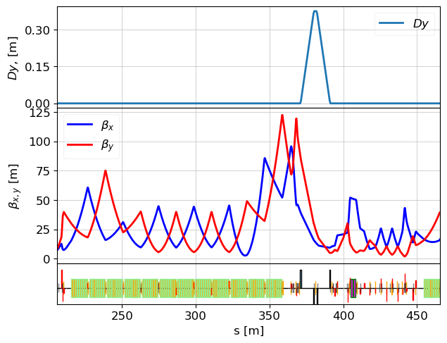
Check Twiss Parameters at Key Elements
We use markers for the TDS and screens (e.g., d_223, otrb_457_b2) and inspect relevant optics values like beta functions and phase advances.
tds_marker = l2.d_223
tws = twiss(lat_l2, tws0=l2.twiss0, attach2elem=True)
# with attach2elem=True to all elements will be attached Twiss object in element.tws
# let's print beta_x
print("TDS center beta_x = ", tds_marker.tws.beta_x)
print("Screen 457 beta_x = ", l2.otrb_457_b2.tws.beta_x)
print("Screen 457 beta_y = ", l2.otrb_457_b2.tws.beta_y)
print("Screen 457 alpha_x = ", l2.otrb_457_b2.tws.alpha_x)
print("Screen 457 alpha_y = ", l2.otrb_457_b2.tws.alpha_y)
print("Phase advance between TDS and screen OTRB.457.B2 = ", ( l2.otrb_457_b2.tws.mux - l2.d_223.tws.mux)/( np.pi) * 180)
_, R, _ = lat_l2.transfer_maps(start=l2.d_223, stop=l2.otrb_457_b2, energy=2.4)
print(f"R12 = {R[0,1]}")
TDS center beta_x =  50.88807908849443
Screen 457 beta_x =  17.046378671795534
Screen 457 beta_y =  5.9780720514095345
Screen 457 alpha_x =  2.134410976038094
Screen 457 alpha_y =  -0.9840253685422208
Phase advance between TDS and screen OTRB.457.B2 =  98.47289527403284
R12 = 29.148479168428796
Define Matching Start and End Points
We preserve Twiss parameters at match_385_b2 (entry point after L2) and stac_477_l3 (end of the matched region).
END_ELEM = l3.stac_477_l3

tws_match_385 = copy.deepcopy(l2.match_385_b2.tws)
tws_end = copy.deepcopy(END_ELEM.tws)
Shorten Lattice to Relevant Region
We exclude upstream quadrupoles and start optimization just after L2.
lat = MagneticLattice(l2.cell+l3.cell, start=l2.match_385_b2, stop=END_ELEM)
tws_des = twiss(lat, tws0=tws_match_385)
plot_opt_func(lat, tws_des, top_plot = ["Dy"], legend=False)
plt.savefig("TDS_area_design.png")
plt.show()
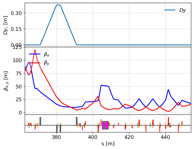
(Optional) Save Quadrupole Strengths for Reference
We optionally store the design quadrupole strengths in a CSV file for comparison later. The function looks a bit complicated just because I wanted to avoid overwriting every time design quads strengths.
# let's save design kicks to a dictionary
df_filename = "quads_strengths.csv"
design_column = "design"
if os.path.exists(df_filename):
    quads_kicks_df = pd.read_csv(df_filename, index_col=0)
    if design_column in quads_kicks_df.columns:
        print(f"Column '{design_column}' already exists. Skipping step.")
    else:
        print(f"Column '{design_column}' not found. Proceeding to add it.")
        quads_kicks_df[design_column] = pd.Series(d_design)
        df.to_csv(df_filename)
else:
    print("File does not exist. Creating new DataFrame.")
    # let's save design kicks to a dictionary
    d_design = {}
    for e in lat.sequence:
        if e.__class__ == Quadrupole:
            d_design[e.id] = e.k1
    quads_kicks_df = pd.DataFrame({design_column: d_design})
    quads_kicks_df.to_csv(df_filename, index=True)
Column 'design' already exists. Skipping step.
Display Twiss Parameters at Specific Elements
We define a helper function to show selected optics values and compute R12 matrix elements.
It can be done in different ways but we will use pandas.
# List of elements where we want to see Twiss parameters
elements_for_comparision = {'TDS 429': tds_marker, "Scr 450": l2.otrb_450_b2,  "Scr 454": l2.otrb_454_b2, 'Scr 457': l2.otrb_457_b2, 'Scr 461': l2.otrb_461_b2, 'end': END_ELEM}

# Attributes we want to compare
attributes = ['beta_x', 'beta_y', 'alpha_x', 'alpha_y', 'mux', "muy"]

def table_update(lat, tws0, elements_for_comparision, attributes):
    # calculate Twiss
    tws = twiss(lat, tws0=tws0, attach2elem=True)

    # Build the table from tws list
    table = pd.DataFrame({name: [getattr(getattr(obj, "tws"), attr) for attr in attributes] for name, obj in elements_for_comparision.items()},
                     index=attributes)
    # make phase advance in degree
    table.loc['mux'] = (table.loc['mux'] - table.loc['mux', 'TDS 429'])*180/np.pi
    table.loc['muy'] = (table.loc['muy'] - table.loc['muy', 'TDS 429'])*180/np.pi
    # add R12 elements into table
    R12_values = copy.copy(elements_for_comparision)
    for key in R12_values:
        stop_elem = elements_for_comparision[key]
        _, R, _ = lat.transfer_maps(energy=2.4, start=tds_marker, stop=stop_elem)
        R12_values[key] = R[0, 1]
    table.loc['R12'] = R12_values
    return table
table = table_update(lat, tws_match_385, elements_for_comparision, attributes)
table
| TDS 429 | Scr 450 | Scr 454 | Scr 457 | Scr 461 | end | |
|---|---|---|---|---|---|---|
| beta_x | 50.888079 | 17.072932 | 16.948653 | 17.046379 | 17.188861 | 17.076953 |
| beta_y | 7.648263 | 5.978131 | 6.051098 | 5.978072 | 5.968185 | 15.300108 |
| alpha_x | 0.224536 | 2.138285 | -2.153417 | 2.134411 | -2.180546 | 0.445896 |
| alpha_y | 0.850922 | -0.984060 | 1.006426 | -0.984025 | 0.985766 | -0.587954 |
| mux | 0.000000 | 71.459877 | 88.165681 | 98.472895 | 115.072173 | 156.350561 |
| muy | 0.000000 | 165.438742 | 192.476386 | 241.936757 | 269.174958 | 405.512304 |
| R12 | 0.400000 | 28.068808 | 29.412231 | 29.148479 | 26.737475 | 11.633821 |
Matching
Objective: High Beta at TDS and 90° Phase Advance to Screen
We now want to modify the optics such that:
- The beta function at the TDS position is large (150 m), which improves time resolution.
- The phase advance between the TDS and screen is exactly 90 degrees.
To achieve this, we define a set of constraints and a list of quadrupoles we allow the matcher to modify.
from ocelot.cpbd.matcher import MatchProblem

problem = MatchProblem(lat, tws_match_385)

# variables
problem.vary_element(l2.qd_417_b2, quantity="k1", limits=(-5, 5))
problem.vary_element(l2.qd_418_b2, quantity="k1", limits=(-5, 5))
problem.vary_element(l2.qd_425_b2, quantity="k1", limits=(-5, 5))
problem.vary_element(l2.qd_427_b2, quantity="k1", limits=(-5, 5))

problem.vary_element(l2.qd_431_b2, quantity="k1", limits=(-5, 5))
problem.vary_element(l2.qd_434_b2, quantity="k1", limits=(-5, 5))
problem.vary_element(l2.qd_437_b2, quantity="k1", limits=(-5, 5))
problem.vary_element(l2.qd_440_b2, quantity="k1", limits=(-5, 5))

problem.vary_element(l2.qd_444_b2, quantity="k1", limits=(-5, 5))
problem.vary_element(l2.qd_448_b2, quantity="k1", limits=(-5, 5))
problem.vary_element(l2.qd_452_b2, quantity="k1", limits=(-5, 5))
problem.vary_element(l2.qd_456_b2, quantity="k1", limits=(-5, 5))

# Twiss targets
problem.target_twiss(tds_marker, "beta_x", 150, weight=1e6)
problem.target_twiss(tds_marker, "alpha_x", 0, weight=1e6)
problem.target_twiss(l2.otrb_457_b2, "beta_x", l2.otrb_457_b2.tws.beta_x, weight=1e6)
problem.target_twiss(l2.otrb_457_b2, "beta_y", l2.otrb_457_b2.tws.beta_y, weight=1e6)
problem.target_twiss(l2.otrb_457_b2, "alpha_x", l2.otrb_457_b2.tws.alpha_x, weight=1e6)
problem.target_twiss(l2.otrb_457_b2, "alpha_y", l2.otrb_457_b2.tws.alpha_y, weight=1e6)


problem.target_twiss_delta(
    start=tds_marker,
    end=l2.otrb_457_b2,
    quantity="mux",
    value=np.pi / 2.0,
    relation="==",
    wrap_phase=True,  # wrap residual to [-pi, pi]
    weight=1e6,
    tol=1e-4,
    name="phase_advance",
)

result = problem.solve(solver="ls_trf", max_iter=300)
print(result.success, result.merit)
tws_hi_res = twiss(lat, tws0=tws_match_385, attach2elem=True)
print(l2.otrb_457_b2.tws)
plot_opt_func(lat, tws_hi_res, top_plot=["Dy"], legend=False)
plt.show()
True 2.3139596185065114e-09
emit_x  = 0.0
emit_y  = 0.0
emit_xn  = 0.0
emit_yn  = 0.0
beta_x  = 17.04637866884113
beta_y  = 5.978072057730435
alpha_x = 2.1344109925101633
alpha_y = -0.9840254089866904
Dx      = -8.045300817594888e-13
Dy      = 5.2074661182796385e-11
Dxp     = -3.8369526413224683e-13
Dyp     = 1.4177277577777732e-11
mux     = 12.713205782912105
muy     = 15.484839848144187
nu_x    = 2.023369542894931
nu_y    = 2.4644888048185014
E       = 2.4000000004506834
s        = 435.069106
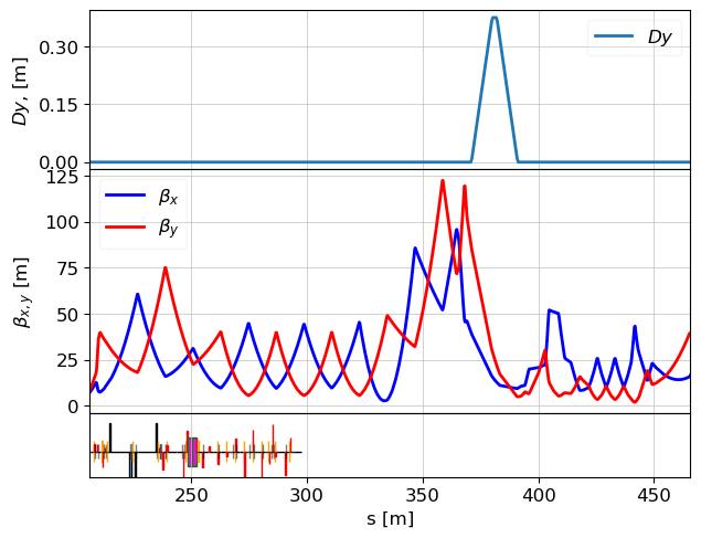
table = table_update(lat, tws_match_385, elements_for_comparision, attributes)
table
| TDS 429 | Scr 450 | Scr 454 | Scr 457 | Scr 461 | end | |
|---|---|---|---|---|---|---|
| beta_x | 150.000000 | 10.690676 | 14.897255 | 17.046379 | 17.188861 | 17.076952 |
| beta_y | 5.867822 | 5.888962 | 6.491762 | 5.978072 | 5.968185 | 15.300108 |
| alpha_x | 0.000000 | 1.123414 | -2.535310 | 2.134411 | -2.180546 | 0.445896 |
| alpha_y | 0.045016 | -1.196312 | 1.144382 | -0.984025 | 0.985766 | -0.587954 |
| mux | 0.000000 | 56.165456 | 79.346153 | 89.998593 | 106.597871 | 147.876259 |
| muy | 0.000000 | 157.440624 | 182.919361 | 231.472815 | 258.711015 | 395.048361 |
| R12 | 0.400000 | 33.322788 | 46.479874 | 50.566364 | 48.622845 | 26.798440 |
Compare design and new optics
bx_n = [tw.beta_x for tw in tws_hi_res]
by_n = [tw.beta_y for tw in tws_hi_res]
s_n = np.array([tw.s for tw in tws_hi_res])
bx_d = [tw.beta_x for tw in tws_des]
by_d = [tw.beta_y for tw in tws_des]
s_d = np.array([tw.s for tw in tws_des])

fig, ax = plot_API(lat, legend=False, figsize=[10,6])

ax.plot(s_n - s_n[0], bx_n, 'C0', label=r"hi res $\beta_{x}$ ")
ax.plot(s_n - s_n[0], by_n, 'C1', label=r"hi res $\beta_{y}$ ")
ax.plot(s_d - s_d[0], bx_d, "C0--", label=r"design $\beta_{x}$ ")
ax.plot(s_d - s_d[0], by_d, "C1--", label=r"design $\beta_{y}$ ")
ax.set_ylabel(r"$\beta_{x,y}$ [m]")
ax.legend()
#plt.savefig("TDS_90m.png")
plt.show()
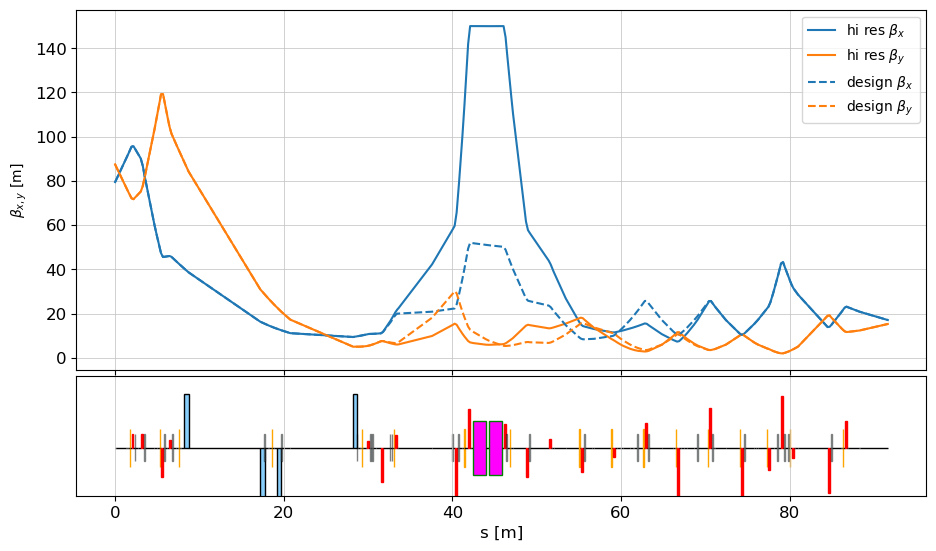
for key in ['beta_x', "beta_y", "alpha_x", "alpha_y"]:
    print(key, " :", getattr(tws_hi_res[-1], key), getattr(tws_des[-1], key))
beta_x  : 17.076952392671416 17.076952650423507
beta_y  : 15.300107642832417 15.300107956262153
alpha_x  : 0.44589593312661785 0.4458959473312124
alpha_y  : -0.5879536113204561 -0.5879535896879575
Write new quadrupole kicks to the dataframe
WRITE_TO_FILE = True
REWRITE = True

beta_tds_ampl = int(round(tds_marker.tws.beta_x))
new_column = f'TDS {beta_tds_ampl}m'


quads_kicks_df = pd.read_csv(df_filename, index_col=0)
# let's save design kicks to a dictionary
d_new = {}
for e in lat.sequence:
    if e.__class__ == Quadrupole:
        d_new[e.id] = e.k1
if WRITE_TO_FILE:
    if new_column in quads_kicks_df.columns and not REWRITE:
        print(f"Column '{new_column}' already exists. Skipping step.")
    else:
        print(f"Column '{new_column}' not found. Proceeding to add it.")
        quads_kicks_df[new_column] = pd.Series(d_new)
        quads_kicks_df.to_csv(df_filename)

quads_kicks_df
Column 'TDS 150m' not found. Proceeding to add it.
| Quad | design | TDS 70m | TDS 90m | TDS 120m | TDS 150m | TDS 200m |
|---|---|---|---|---|---|---|
| QD.387.B2 | 0.335173 | 0.335173 | 0.335173 | 0.335173 | 0.335173 | 0.335173 |
| QD.388.B2 | 0.355996 | 0.355996 | 0.355996 | 0.355996 | 0.355996 | 0.355996 |
| QD.391.B2 | -0.725525 | -0.725525 | -0.725525 | -0.725525 | -0.725525 | -0.725525 |
| QD.392.B2 | 0.196996 | 0.196996 | 0.196996 | 0.196996 | 0.196996 | 0.196996 |
| QD.415.B2 | 0.180686 | 0.180686 | 0.180686 | 0.180686 | 0.180686 | 0.180686 |
| QD.417.B2 | -0.750235 | -0.786614 | -0.885369 | -0.948106 | -0.861790 | -1.043530 |
| QD.418.B2 | 0.649193 | 0.581958 | 0.575173 | 0.494175 | 0.314098 | 0.333096 |
| QD.425.B2 | -1.300803 | -1.322190 | -1.395390 | -1.326928 | -1.251134 | -1.350696 |
| QD.427.B2 | 0.941484 | 0.951529 | 0.992650 | 0.983920 | 0.972917 | 1.021064 |
| QD.431.B2 | 0.435183 | 0.617682 | 0.558198 | 0.640692 | 0.601176 | 0.649302 |
| QD.434.B2 | -0.527858 | -0.748168 | -0.650429 | -0.771803 | -0.730839 | -0.774303 |
| QD.437.B2 | 0.405549 | 0.076025 | 0.274685 | 0.047672 | 0.226122 | 0.014847 |
| QD.440.B2 | -0.668525 | -0.245049 | -0.804925 | -0.245927 | -0.614961 | -0.168753 |
| QD.444.B2 | -0.458219 | -0.811179 | -0.139235 | -0.804551 | -0.223309 | -0.842423 |
| QD.448.B2 | 0.896096 | 0.997524 | 0.732375 | 0.934983 | 0.616211 | 0.831219 |
| QD.452.B2 | -1.263284 | -1.280166 | -1.331850 | -1.451828 | -1.352353 | -1.578397 |
| QD.456.B2 | 0.896096 | 0.850322 | 0.947912 | 0.957766 | 1.009984 | 1.039100 |
| QD.459.B2 | -1.263284 | -1.263284 | -1.263284 | -1.263284 | -1.263284 | -1.263284 |
| QD.463.B2 | -0.569607 | -0.569607 | -0.569607 | -0.569607 | -0.569607 | -0.569607 |
| QD.464.B2 | 1.298268 | 1.298268 | 1.298268 | 1.298268 | 1.298268 | 1.298268 |
| QD.465.B2 | -0.246861 | -0.246861 | -0.246861 | -0.246861 | -0.246861 | -0.246861 |
| QD.470.B2 | -1.128907 | -1.128907 | -1.128907 | -1.128907 | -1.128907 | -1.128907 |
| QD.472.B2 | 0.661180 | 0.661180 | 0.661180 | 0.661180 | 0.661180 | 0.661180 |
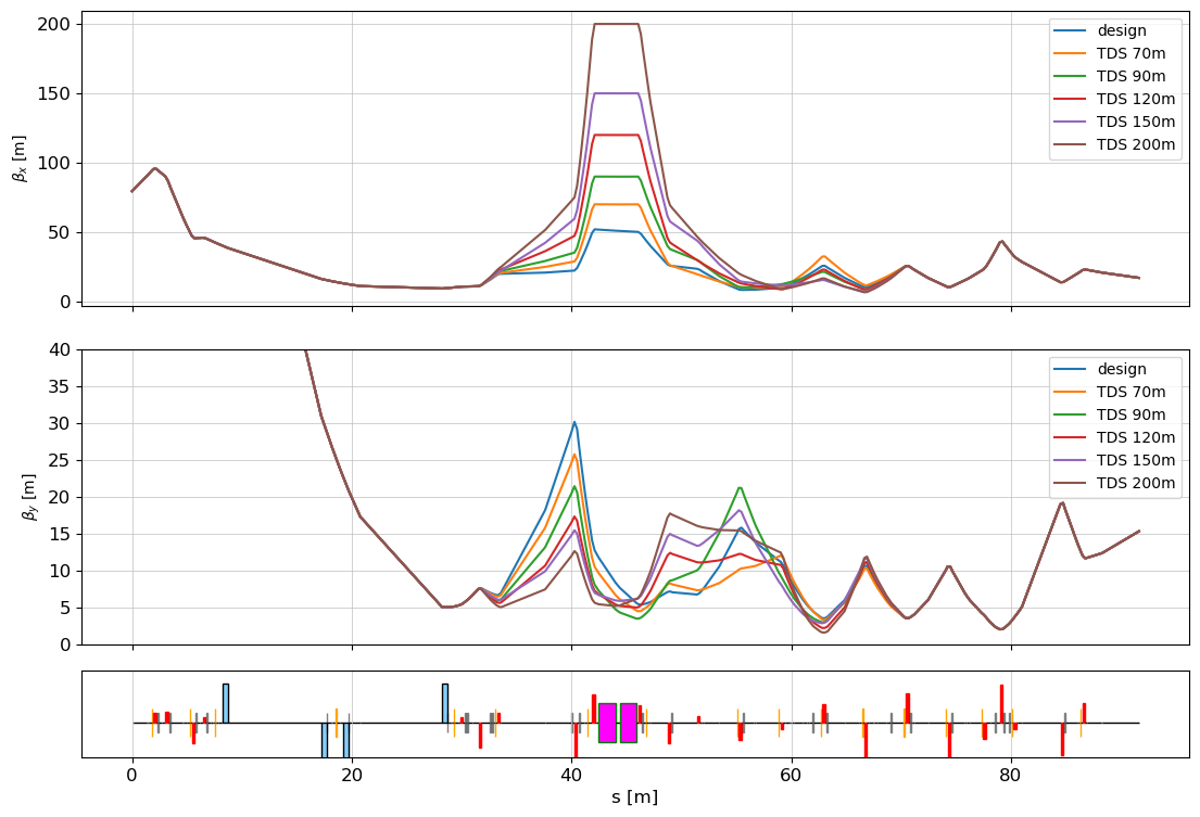
Check optics again from dataframe
quads_kicks_df = pd.read_csv(df_filename, index_col=0)
quads = list(quads_kicks_df.index)
optics = list(quads_kicks_df.columns)
#optics.remove('TDS 70m')
#optics.remove('TDS 120m')
fig, (ax_extra, ax_xy) = plot_API(lat, figsize=(12,8), add_extra_subplot=True, legend=False)
ax_extra.set_ylabel(r"$\beta_x$ [m]")
ax_xy.set_ylabel(r"$\beta_y$ [m]")
data = {}
for opt in optics:
    data[opt] = []
    for e in lat.sequence:
        if e.id in quads:
            e.k1 = quads_kicks_df[opt][e.id]

    tws = twiss(lat, tws0=tws_match_385)
    data[opt] = tws
    s = np.array([tw.s for tw in tws]) - tws[0].s
    bx = [tw.beta_x for tw in tws]
    by = [tw.beta_y for tw in tws]
    ax_extra.plot(s, bx, label=opt)
    ax_xy.plot(s, by, label=opt)
    ax_xy.set_ylim([0,40])
ax_xy.legend()
ax_extra.legend()
plt.show()
Let’s Put Some Numbers to Understand the TDS Voltage (Streaking/Calibration Factor)
The streaking factor is given by:
or, as defined above, it can be rewritten using the transfer matrix element:
During an experimental study of the proposed optics with a 150 m beta function, we measured a calibration factor of mm/ps for our S-band TDS (operating at 3 GHz). For optics TDS150m, we have between the TDS and a screen (Scr 457). Let’s calculate the required TDS voltage:
f = 3e9 # [Hz] frequency of the S-band TDS
S = 11.1e-3/1e-12 # [mm/ps] → [m/s]
R12 = 50
Lrf = speed_of_light /f
pc = 2400 # [MeV]

V = S * Lrf * pc /(R12 * 2 * np.pi* speed_of_light)
print(f"TDS voltage = {V} MV")
TDS voltage = 28.26591789312062 MV
Let's estimate time resolution
We performed another measurement on a different day, when the TDS voltage was slightly lower, using standard optics. The time resolution was measured to be about 11 fs.
f = 3e9 # [Hz] frequency of the S-band TDS
emitt = 0.5e-6  # normalized m
E = 2.4         # GeV
k = 2 * np.pi/speed_of_light*f         # 1/m
V = 0.024        # GV
beta_tds = 50   # m
beta_scr = 17 # m
phi = 98.7 * np.pi/180
gamma = E/m_e_GeV
sigma_scr  = np.sqrt(beta_scr*emitt/gamma)  # m
print(f"sigma = {sigma_scr} m")
S = np.sqrt(beta_tds*beta_scr) * np.sin(phi) * speed_of_light*k * V/E
print(f"S = {S} m/s")
print(f"S = {S*1e-12/1e-3} mm/ps - this is what we measure typically during time calibration")
print(f"R = {sigma_scr/S*1e15} fs - we measured 11 fs")
sigma = 4.2541599106903523e-05 m
S = 5432310354.635417 m/s
S = 5.432310354635416 mm/ps - this is what we measure typically during time calibration
R = 7.8312166149716695 fs - we measured 11 fs