This notebook was created by Sergey Tomin (sergey.tomin@desy.de). April 2025.
Ocelot for Students
This tutorial is aimed
at students and beginners in accelerator physics.
The idea is to keep it simple and interactive, helping you build intuition about how magnetic elements work.
Quadrupole Doublet
In this section, we will consider a simple beamline consisting of only a drift and two quadrupoles.
As usual, let's import the necessary Ocelot modules, the standard Python copy library, and ipywidgets for interaction with the physics model.
💡 Tip: If you don't have the
ipywidgetsmodule installed, just search online for installation instructions:pip install ipywidgets
Create a Simple Lattice
d = Drift(l=1.)
qf = Quadrupole(l=0.2, k1=1)
qd = Quadrupole(l=0.2, k1=-1)
cell = [d, qf, d, qd, d]

lat = MagneticLattice(cell)
Plot Beta Functions
Now we define a function that calculates and plots the beta functions for a simple lattice with a focusing and defocusing quadrupole.
You can interactively change the quadrupole strengths using sliders (if using ipywidgets), and observe how the beta functions evolve.
def plot_betas(qf_k1=1.0, qd_k1=-1.0, save_path=None):
    # Set quadrupole strengths
    qf.k1 = qf_k1
    qd.k1 = qd_k1

    # Define initial Twiss parameters
    tws0 = Twiss(beta_x=10, beta_y=10, alpha_x=0, alpha_y=0)

    # Calculate Twiss parameters along the beamline
    tws = twiss(lat, tws0, nPoints=20)

    # Extract s-position and beta functions
    sb = [tw.s for tw in tws]
    bx = [tw.beta_x for tw in tws]
    by = [tw.beta_y for tw in tws]

    # Plot using Ocelot's built-in function (you can also use matplotlib directly)
    fig, ax_xy = plot_API(lat, fig_name=f"Beta-functions: QF.k1={qf_k1:.2f}, QD.k1={qd_k1:.2f}", legend=False)
    fig.suptitle(f"Beta-functions: QF.k1={qf_k1:.2f}, QD.k1={qd_k1:.2f}")

    ax_xy.plot(sb, bx, "C1", label=r"$\beta_x$")
    ax_xy.plot(sb, by, "C2", label=r"$\beta_y$")
    ax_xy.set_ylabel(r"$\beta_{x,y}$ [m]")
    ax_xy.set_xlabel("S [m]")
    ax_xy.legend()
    if save_path:
        fig.savefig(save_path)
        plt.close(fig)
    else:
        plt.show()
Interactive widget:
# Create interactive sliders for the parameters
interact(
    lambda qf_k1,qd_k1: plot_betas(qf_k1,qd_k1, save_path=None),
    qf_k1=FloatSlider(min=-20, max=20, step=0.1, value=1.0),
    qd_k1=FloatSlider(min=-20, max=20, step=0.1, value=-1.0),
)

Plot Trajectories for Better Understanding of Transverse Beam Dynamics
Now let's plot particle trajectories with initial transverse offsets to better visualize how the beam evolves through the lattice.
We’ll use two subplots: one for horizontal (x) and one for vertical (y) motion.
def plot_beam(qf_k1=1.0, qd_k1=-1.0, save_path=None):
    qf.k1 = qf_k1
    qd.k1 = qd_k1

    x_coors = np.linspace(-0.01, 0.01, num=10)
    y_coors = np.linspace(-0.01, 0.01, num=10)

    p_list = [Particle(x=x, y=y) for x, y in zip(x_coors, y_coors)]
    P = [copy.deepcopy(p_list)]
    navi = Navigator(lat)
    dz = 0.01

    for _ in range(int(lat.totalLen / dz)):
        tracking_step(lat, p_list, dz=dz, navi=navi)
        P.append(copy.deepcopy(p_list))
    fig, (ax_x, ax_y) = plot_API(lat, figsize=(10,6), legend=False, add_extra_subplot=True)
    fig.suptitle(f"Particle Trajectories with Transverse Offsets: QF.k1={qf_k1:.2f}, QD.k1={qd_k1:.2f}")

    for i in range(len(p_list)):
        s = [p[i].s for p in P]
        x = [p[i].x for p in P]
        y = [p[i].y for p in P]
        ax_x.plot(s, x, "C0")
        ax_y.plot(s, y, "C1")

    ax_x.set_ylabel("X [m]")
    ax_y.set_ylabel("Y [m]")
    ax_x.grid(True)
    ax_y.grid(True)
    if save_path:
        fig.savefig(save_path)
        plt.close(fig)
    else:
        plt.show()
Add the interactive widget:
# Create interactive sliders for the parameters
interact(
    lambda qf_k1,qd_k1: plot_beam(qf_k1,qd_k1, save_path=None),
    qf_k1=FloatSlider(min=-20, max=20, step=0.1, value=1.0),
    qd_k1=FloatSlider(min=-20, max=20, step=0.1, value=-1.0),
)

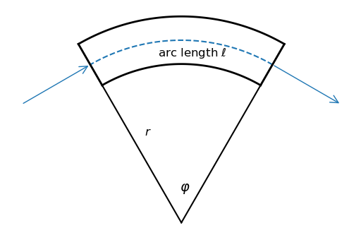
Bending Magnet: Quick Look at Dispersion
Let's take a look at transverse beam dynamics in a dipole magnet.
A Simple Lattice
We define a basic beamline composed of a drift–dipole–drift sequence:
d = Drift(l=1)
b1 = Bend(l=0.5, angle=5/180*np.pi, e1=0, e2=0)
cell = [d, b1, d]
lat2 = MagneticLattice(cell)
Dispersion Visualization
Now we’ll create particles with zero initial transverse coordinates, but different momentum deviations, and observe how this affects their horizontal position. In other words, we’ll see dispersion in action 😊
def plot_dipole_disp(angle=0.01, save_path=None):
    # Set dipole parameters (angle in degrees -> radians)
    b1.angle = angle * np.pi / 180
    b1.e1 = 0 # edge focusing is 0 Basically it is SBend magnet
    b1.e2 = 0 # edge focusing is 0 Basically it is SBend magnet
    print(f"Lattice length: {lat2.totalLen:.2f} m")

    # Create particles with momentum deviations (x = 0, y = 0)
    p_coors = np.linspace(-0.01, 0.01, num=10)
    p_list = [Particle(x=0, y=0, p=p, E=1) for p in p_coors]
    P = [copy.deepcopy(p_list)]

    # Navigator and tracking step size
    navi = Navigator(lat2)
    dz = 0.01

    # Track particles through the lattice
    for _ in range(int(lat2.totalLen / dz)):
        tracking_step(lat2, p_list, dz=dz, navi=navi)
        P.append(copy.deepcopy(p_list))

    # Plot horizontal trajectories and momenta
    fig, (ax_x, ax_p) = plot_API(lat2, figsize=(10,6), legend=False, add_extra_subplot=True)

    fig.suptitle(f"Effect of Dispersion in a Dipole Magnet: Angle = {angle:.1f}")

    colors = plt.cm.rainbow(np.linspace(0, 1, len(p_list)))[::-1]
    for i in range(len(p_list)):
        s = [p[i].s for p in P]
        x = [p[i].x for p in P]
        p_vals = [p[i].p for p in P]

        ax_x.plot(s, x, color=colors[i])
        ax_p.plot(s, p_vals, color=colors[i])

    ax_x.set_ylabel("X [m]")
    ax_p.set_ylabel("Relative Momentum p")
    ax_x.set_ylim([-0.005, 0.005])

    ax_x.grid(True)
    ax_p.grid(True)
    if save_path:
        fig.savefig(save_path)
        plt.close(fig)
    else:
        plt.show()
Widget:
# Create interactive sliders for the parameters
interact(
    lambda angle: plot_dipole_disp(angle=angle, save_path=None),
    angle=FloatSlider(min=-30, max=30, step=0.05, value=1.0),
)
Do Bending Magnets Focus the Beam?
In this section, we investigate whether bending magnets can provide transverse focusing. We'll compare two common types of dipole magnets used in accelerator physics: the sector dipole magnet (SBend) and the rectangular dipole magnet (RBend). Each has distinct edge geometries, which affect how the beam is focused or defocused in the transverse plane.
Sector Dipole Magnet (SBend)
A sector dipole has its entrance and exit faces aligned perpendicular to the reference trajectory.
In the animation below, you can see how a beam propagates through an SBend, and how the transverse position evolves due to the edge focusing.
# Assuming these come from your simulation code
# from your_code import Drift, SBend, MagneticLattice, Navigator, Particle, tracking_step

# Setup lattice (this stays outside the function)
d = Drift(l=1)
b = SBend(l=0.5, angle=5/180*np.pi)
cell = [d, b, d]
lat3 = MagneticLattice(cell)

def plot_sbend_focus(angle=0.01, save_path=None):
    b.angle = angle * np.pi / 180
    b.e1 = 0
    b.e2 = 0
    x_coors = np.linspace(-0.01, 0.01, num=10)
    p_list = [Particle(x=x, y=x, p=0, E=1) for x in x_coors]
    P = [copy.deepcopy(p_list)]

    navi = Navigator(lat3)
    dz = 0.01

    for _ in range(int(lat3.totalLen / dz)):
        tracking_step(lat3, p_list, dz=dz, navi=navi)
        P.append(copy.deepcopy(p_list))
    fig, (ax_x, ax_y) = plot_API(lat3, figsize=(10,6), legend=False, add_extra_subplot=True)
    fig.suptitle(f"Sector Magnet: Focusing  Effect: Angle = {angle:.1f}°")

    for i in range(len(p_list)):
        s = [p[i].s for p in P]
        x = [p[i].x for p in P]
        y = [p[i].y for p in P]

        ax_x.plot(s, x, "C0")
        ax_y.plot(s, y, "C1")

    ax_x.set_ylabel("X [m]")
    ax_y.set_ylabel("Y [m]")
    ax_x.grid(True)
    ax_y.grid(True)

    if save_path:
        fig.savefig(save_path)
        plt.close(fig)
    else:
        plt.show()

# Create interactive sliders for the parameters
interact(
    lambda angle: plot_sbend_focus(angle=angle, save_path=None),
    angle=FloatSlider(min=-90, max=90, step=1, value=0),)
Rectangular Dipole Magnet (RBend)
The rectangular dipole is simpler and more common in practice due to ease of manufacturing. Unlike the SBend, in a rectangular dipole the entrance and exit faces are perpendicular to the magnet body, not to the beam trajectory. As a result, the beam enters and exits the magnet at an angle of with respect to the face of the magnet, where is the total bending angle.
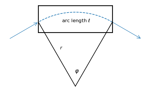
The animation below demonstrates how a beam behaves when passing through an RBend, illustrating the distinct focusing effect caused by the non-normal incidence at the edges.
# Assuming these come from your simulation code
# from your_code import Drift, SBend, MagneticLattice, Navigator, Particle, tracking_step

# Setup lattice (this stays outside the function)
d = Drift(l=1)
b = RBend(l=0.5, angle=5/180*np.pi)
cell = [d, b, d]
lat3 = MagneticLattice(cell)

def plot_rbend_focus(angle=0.01, save_path=None):
    b.angle = angle * np.pi / 180
    b.e1 = b.angle/2 # edge angle is not changing automatcally it has to be also set
    b.e2 = b.angle/2 # edge angle is not changing automatcally it has to be also set

    x_coors = np.linspace(-0.01, 0.01, num=10)
    p_list = [Particle(x=x, y=x, p=0, E=1) for x in x_coors]
    P = [copy.deepcopy(p_list)]

    navi = Navigator(lat3)
    dz = 0.01

    for _ in range(int(lat3.totalLen / dz)):
        tracking_step(lat3, p_list, dz=dz, navi=navi)
        P.append(copy.deepcopy(p_list))

    fig, (ax_x, ax_y) = plot_API(lat3, figsize=(10,6), legend=False, add_extra_subplot=True)
    fig.suptitle(f"Rectangular Magnet: Focusing  Effect: Angle = {angle:.1f}°")

    for i in range(len(p_list)):
        s = [p[i].s for p in P]
        x = [p[i].x for p in P]
        y = [p[i].y for p in P]

        ax_x.plot(s, x, "C0")
        ax_y.plot(s, y, "C1")

    ax_x.set_ylabel("X [m]")
    ax_y.set_ylabel("Y [m]")
    ax_x.grid(True)
    ax_y.grid(True)
    #plt.tight_layout(rect=[0, 0.03, 1, 0.95])

    if save_path:
        fig.savefig(save_path)
        plt.close(fig)
    else:
        plt.show()

# Create interactive sliders for the parameters
interact(
    lambda angle: plot_rbend_focus(angle=angle, save_path=None),
    angle=FloatSlider(min=-90, max=90, step=1, value=0),)