This notebook was created by Sergey Tomin (sergey.tomin@desy.de) who was inspired by questions from E.R. June 2017.

Tutorial N7: Lattice Design, Matching, and Twiss Backtracking

Outline

• Design of a FODO lattice (undulator section) with specified maximum and minimum Twiss parameters
• Backtracking through chicanes
• Matching Twiss parameters in matching sections

---

Introduction

In this tutorial, we design a basic FEL beamline for an external seeding configuration. The layout consists of:

• Matching section
• Modulator – Chicane – Modulator – Chicane
• FODO lattice (undulator section)

The FODO section consists of repeating cells:

• undulator – QF – undulator – QD – undulator – QF – ...

where QF and QD are focusing and defocusing quadrupoles, respectively.

We assume that:

1. The maximum and minimum values of the beta functions in the undulator section are known
2. The chicane geometry and parameters are predefined
3. The Twiss parameters at the entrance of the matching section are given

While this problem can be solved in multiple (and possibly simpler) ways, we take a structured approach to demonstrate the use of Ocelot’s matching and backtracking tools:

1. Match Twiss parameters within the FODO lattice to reach desired beta amplitudes using the match function
2. Perform Twiss backtracking through the chicanes and modulators using the twiss function
3. Use the MagneticLattice class to construct the full lattice

---

Optics Design and Matching

Optics design is still something of an art — and only a few people in the world truly excel at it
(and the author of this notebook is certainly not one of them — at least not yet! :) ).

This tutorial is not aimed at producing an optimal design, but rather to illustrate the use of Ocelot’s matching functions in a practical setting.

# the output of plotting commands is displayed inline within 
# frontends, directly below the code cell that produced it.
%matplotlib inline

from time import time 

# this python library provides generic shallow (copy) 
# and deep copy (deepcopy) operations 
from copy import deepcopy

# import from Ocelot main modules and functions
from ocelot import *

# import from Ocelot graphical modules
from ocelot.gui.accelerator import *

    initializing ocelot...

Step 1. FODO lattice matching

Design the simplest FODO lattice

# example of the FODO
U = Undulator(nperiods=50, lperiod=0.04, Kx=1)
D = Drift(l=0.5)
QF = Quadrupole(l=0.25, k1=1)
QD = Quadrupole(l=0.25, k1=-1)

M1 = Marker()
cell = (M1, QF, D, U, D, QD, QD, D, U, D, QF)

# suppose we have 5 cells or 10 undulators
fodo = cell*5

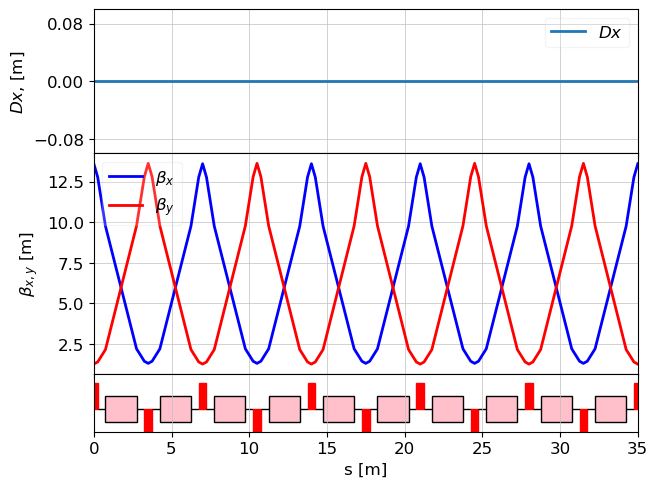
Periodic solution for FODO lattice

Note

• In the most cases to find twiss periodical solution we do not need to put the initial conditions and we can use following command to calculate twiss parameters: tws = twiss(lat)

BUT

• To take into account undulator vertical focusing effect we have to define the energy of the electron beam. and in that case we have to define initial condition like that:

# create MagneticLattice object
lat_fodo = MagneticLattice(fodo)

tws0 = Twiss()
# by default the all parameters are zero and 
# that what we need to force the twiss function 
# to calculate periodic solution

# print(tws0)

# And we need to define the beam energy
tws0.E = 1 # GeV

tws = twiss(lat_fodo, tws0=tws0)

plot_opt_func(lat_fodo, tws, legend=False)
plt.show()

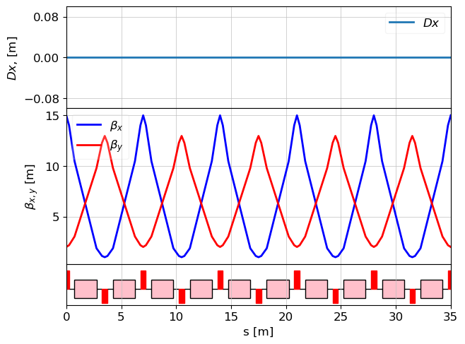
Matching

In Ocelot there is function match() to perform some standard matching procedures.

def match(lat, constr, vars, tw):
    ...
    return res

where

• lat: MagneticLattice

• constr: dictionary, constrains. Example:

  • 'periodic':True - means the "match" function tries to find periodic solution at the ends of lattice:

    constr = {elem1:{'beta_x':15, 'beta_y':2}, 'periodic':True}

  • "hard" constrains on the end of elements (elem1, elem2):

    constr = {elem1:{'alpha_x':5, 'beta_y':5}, elem2:{'Dx':0 'Dyp':0, 'alpha_x':5, 'beta_y':5}}

  • or mixture of "soft" and hard constrains:

    constr = {elem1:{'alpha_x':[">", 5], 'beta_y':5}, elem2:{'Dx':0 'Dyp':0, 'alpha_x':5, 'beta_y':[">", 5]}}

  • in case one needs global control on beta function, the constrains can be written following way.

    constr = {elem1:{'alpha_x':5, 'beta_y':5}, 'global': {'beta_x': ['>', 10]}}

• vars: list of elements which will be varied during optimization, e.g. vars = [QF, QD]

  can be

  • Quadrupole (vary strength 'k1'),
  • SBend, RBend, Bend (by default vary 'k1' but can be "angle"),
  • Solenoid (vary strength "k"),
  • Drift (vary length "l")

• tw: Twiss(), initial Twiss

Optional arguments:

• verbose: True, allow print output of minimization procedure
• max_iter: 1000, number of iterations
• method: string, available 'simplex', 'cg', 'bfgs'
• weights: function returns weights, for example
  def weights_default(val): if val == 'periodic': return 10000001.0 if val == 'total_len': return 10000001.0 if val in ['Dx', 'Dy', 'Dxp', 'Dyp']: return 10000002.0 if val in ['alpha_x', 'alpha_y']: return 100007.0 if val in ['mux', 'muy']: return 10000006.0 if val in ['beta_x', 'beta_y']: return 100007.0 return 0.0001

• vary_bend_angle: False, allow to vary "angle" of the dipoles instead of the focusing strength "k1"
• min_i5: False, minimization of the radiation integral I5. Can be useful for storage rings optimizations.
• return result

# constrains
constr = {M1:{'beta_x':15, 'beta_y':2}, 'periodic':True}

# variables
vars = [QF, QD]

# initial condition for twiss
tw0=tws[-1]

match(lat_fodo, constr, vars, tw0, verbose=False)

# results 
print("QF.k1 = ", QF.k1)
print("QD.k1 = ", QD.k1)


tws0=Twiss()
tws0.E = 1 # GeV

tws = twiss(lat_fodo, tws0=tws0)

# let's variable *tws_fodo* will be the twiss 
# parameters on the FODO entrance 
tws_fodo = tws[-1]

plot_opt_func(lat_fodo, tws, legend=False)
plt.show()

    initial value: x =  [1, -1]
    Optimization terminated successfully.
             Current function value: 0.000017
             Iterations: 42
             Function evaluations: 82
    QF.k1 =  1.071039959675296
    QD.k1 =  -0.8579474979724729

Step 2. Chicanes.

# undulator + chicane + undulator + chicane
modulator = Undulator(nperiods=10, lperiod=0.1, Kx = 2)

# Chicane from CSR example with small modifications 

b1 = Bend(l = 0.5, angle=-0.0336, e1=0.0, e2=-0.0336, gap=0, tilt=0, eid='BB.393.B2')
b2 = Bend(l = 0.5, angle=0.0336, e1=0.0336, e2=0.0, gap=0, tilt=0,  eid='BB.402.B2')
b3 = Bend(l = 0.5, angle=0.0336, e1=0.0, e2=0.0336, gap=0, tilt=0, eid='BB.404.B2')
b4 = Bend(l = 0.5, angle=-0.0336, e1=-0.0336, e2=0.0, gap=0, tilt=0, eid='BB.413.B2')

d = Drift(l=1.5/np.cos(b2.angle))

start_csr = Marker()
stop_csr = Marker()

# define chicane frome the bends and drifts
chicane = [start_csr, Drift(l=1), b1, d, b2, 
           Drift(l=1.5), b3, d, b4, Drift(l= 1.), stop_csr]


# For sake of buity add randomly couple of the quadrupoles

D1 = Drift(l=0.5)
echo = (D1, QF, D1, modulator, D1, QD, chicane,  QF, D1, modulator,D1, QD, chicane)

Chicane parameters

For example, one wants to know R56 of the whole chicane. It can be easily calculated

lat_chic = MagneticLattice(chicane)
# in that case energy is not important we do not have 
# energy dependant elements here
R = lattice_transfer_map(lat_chic, energy=0)
print("R56 = ", R[4,5]*1000, "mm")

    R56 =  -4.1443249349333655 mm

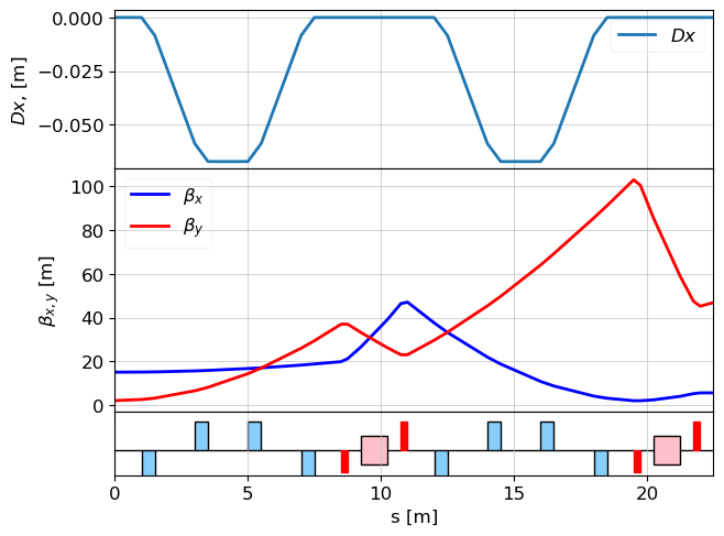
Backtracking though chicanes.

We know twiss parameters on the entrance of the FODO but for backtracking we need to

• invert alphas
• and invert the lattice (change the order of the element)

# inverting alphas

tws2 = Twiss()
tws2.alpha_x = -tws_fodo.alpha_x
tws2.alpha_y = -tws_fodo.alpha_y
tws2.beta_x = tws_fodo.beta_x
tws2.beta_y = tws_fodo.beta_y

# invert the lattice
echo_inv = echo[::-1]
lat_echo_inv = MagneticLattice(echo_inv)

# calculate twiss 
tws_echo = twiss(lat_echo_inv, tws0=tws2)
tws_echo_inv_end = tws_echo[-1]

# show the twiss parameters of INVERTED echo
plot_opt_func(lat_echo_inv, tws_echo, legend=False)
plt.show()

So twiss parameters on the entrance of the echo lattice are:

# inverting alphas again is needed
tws_e = Twiss()
tws_e.beta_x = tws_echo_inv_end.beta_x
tws_e.beta_y = tws_echo_inv_end.beta_y
tws_e.alpha_x = -tws_echo_inv_end.alpha_x
tws_e.alpha_y = -tws_echo_inv_end.alpha_y

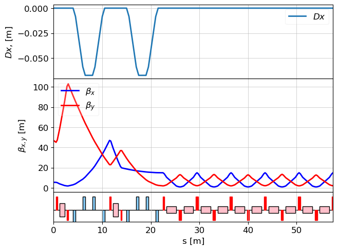
lat_echo_fodo = MagneticLattice((echo, fodo) )

tws_all = twiss(lat_echo_fodo, tws_e)

plot_opt_func(lat_echo_fodo, tws_all, legend=False)
plt.show()

Step 3. Matching section

Q1 = Quadrupole(l=0.3, k1=1)
Q2 = Quadrupole(l=0.3, k1=1)
Q3 = Quadrupole(l=0.3, k1=1)
Q4 = Quadrupole(l=0.3, k1=1)


m1 = Marker()
m2 = Marker()
dm = Drift(l=1.5)
match_sec = (m1, dm, Q1, dm, Q2, dm, Q3, dm, Q4, dm, m2)

lat_m = MagneticLattice(match_sec[::-1])

Matching

As it was mentioned above, matching will not give you desired values if your geometry of initial conditions are poor. Because our goal is not a good design but showing the concept of OCELOT usage, we choose very relax condition. Twiss parameters on the entrance of the matching section:

• beta_x = 5
• beta_y = 5
• alpha_x = not defined
• alpha_y = not defined

the twiss parameters on the exit of matching section are defined by echo section

# constrains
constr = {m1:{'beta_x':5, 'beta_y':5}, 
          m2:{'beta_x':tws_e.beta_x, 'beta_y':tws_e.beta_y, 
              'alpha_x': -tws_e.alpha_x, "alpha_y":-tws_e.alpha_y}}

# variables
vars = [Q1, Q2, Q3,Q4]

# initial condition for twiss

match(lat_m, constr, vars, tw0, verbose=False)

for i, q in enumerate(vars):
    print("Q"+str(i+1)+".k1 = ", q.k1)

tws0 = Twiss()
tws0.beta_x = tws_e.beta_x
tws0.beta_y = tws_e.beta_y
tws0.alpha_x = -tws_e.alpha_x
tws0.alpha_y = -tws_e.alpha_y

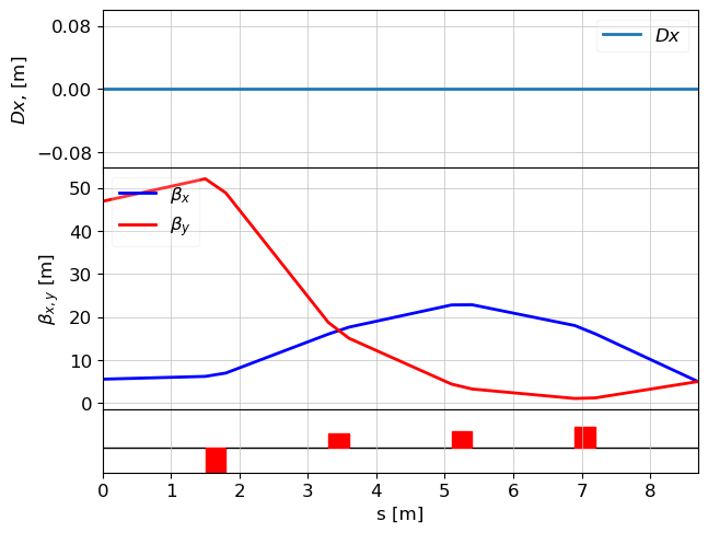
tws = twiss(lat_m, tws0)
plot_opt_func(lat_m, tws, legend=False)
plt.show()

tws0 = tws[-1]
tws0.alpha_x = -tws[-1].alpha_x
tws0.alpha_y = -tws[-1].alpha_y

    initial value: x =  [1, 1, 1, 1]
    Optimization terminated successfully.
             Current function value: 214917575.120251
             Iterations: 106
             Function evaluations: 197
    Q1.k1 =  2.355853351631101
    Q2.k1 =  -1.3155292135369026
    Q3.k1 =  -0.9164603176527466
    Q4.k1 =  1.332649679467849

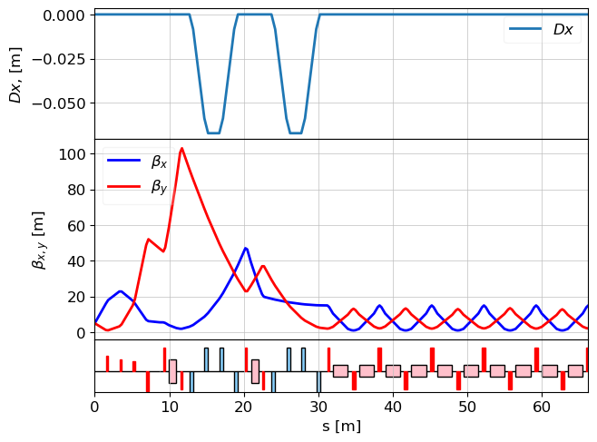
FINAL Lattice

cell = (match_sec, echo, fodo)
# fodo quadrupoles

lat = MagneticLattice(cell)

tws = twiss(lat, tws0)
plot_opt_func(lat, tws, legend=False)
plt.show()